Introducing Goal Seeking into the Segregated Solver

One of the core technologies within the COMSOL Multiphysics® software is the segregated solution approach, which is used within nonlinear multiphysics (and single-physics) problems to rapidly converge to a solution. Did you know it is possible to augment this solver with an additional global equation that can be used to adjust a model input to achieve a desired output? Let’s find out more!

Accelerating Solver Convergence

Whenever you are working on a multiphysics problem, you are solving a system of nonlinear equations. This system of equations is usually quite large, meaning it will take a lot of time, and computational resources, to solve.

One approach to accelerate the convergence of the solver is to use a so-called segregated solver. This solver takes the entire large system of equations, or matrix of equations, and breaks it up (or segregates) into several smaller matrices. Usually, each of these submatrices corresponds to a single physics. During the solution approach, the software will solve one of these submatrices in a so-called segregated step. After stepping through all of the submatrices, the solver will check for convergence and keep iterating as necessary until convergence is achieved.

This approach works robustly for a wide class of problems, is particularly attractive for 3D models that have high computational requirements, and is almost always the default in those cases.

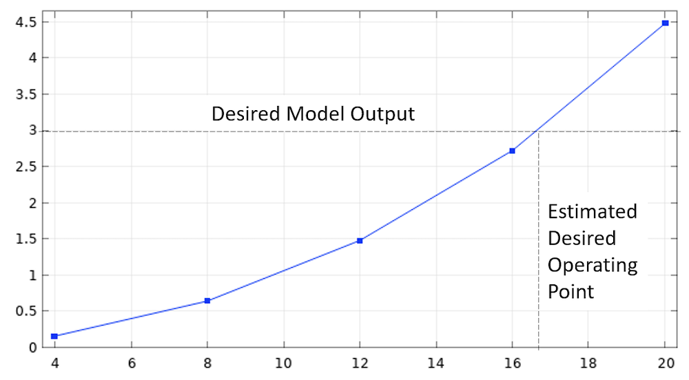
A sweep over a range of input values can be used to predict the model response and estimate the desired operating point.

Often, when solving models, we are in a situation where we don’t want to change the geometry at all, but do want to change some other model input with a single specific goal in mind. That is, we want the model to produce a particular output.

For example, we might want to achieve a desired temperature, heat load, flow rate, or any other derived value. Formally speaking, this is an optimization problem that can easily be addressed using the Optimization Module. However, for the case of only a single model input to vary, using the Optimization Module can be a bit of overkill and we will here look at a few alternative approaches to adjusting an input to get a desired output.

The simplest way of finding this model input is via a parametric sweep. That is, we specify the input that we want to change, give a range of values to sweep over, and then plot the resultant graph of our output vs. input. From this graph, we can visually select the operating point that we are trying to get to.

This is a quite traditional approach, but it is somewhat expensive. Often, the response curves are quite nonlinear, albeit usually monotonic, so you usually need to solve for significantly more than two values within your range of interest, and the solution time will scale with the number of values that you’re solving for. (There is a caveat to this: You can use the Cluster Sweep or Batch Sweep functionalities, but both of these require substantial hardware resources, and this blog post will assume we have some hardware constraints.)

Using a Goal-Seeking Global Equation

Today, let’s look at an alternative, and very efficient, approach to this problem. We will introduce a goal-seeking equation into the segregated solver. This can be done quite simply with:

• A single Global ODE and DAEs interface
• A bit of careful construction of an equation
• Some tweaks to the solver settings

Let’s look at a representative example.

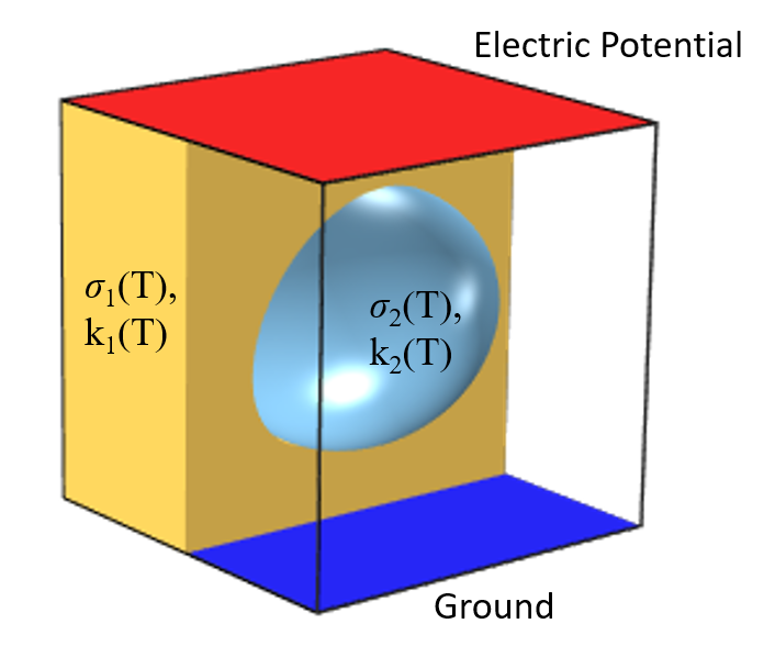
Schematic of a Joule heating problem, an inclusion in the material between two electrodes. All material properties are functions of temperature.

Consider the Joule heating problem illustrated above: two electrodes applied to a medium that contains an inclusion of different conductivity, as might arise in a tissue ablation model. Due to temperature nonlinearities that we will consider in the material properties, such a model can actually produce some quite complicated results.

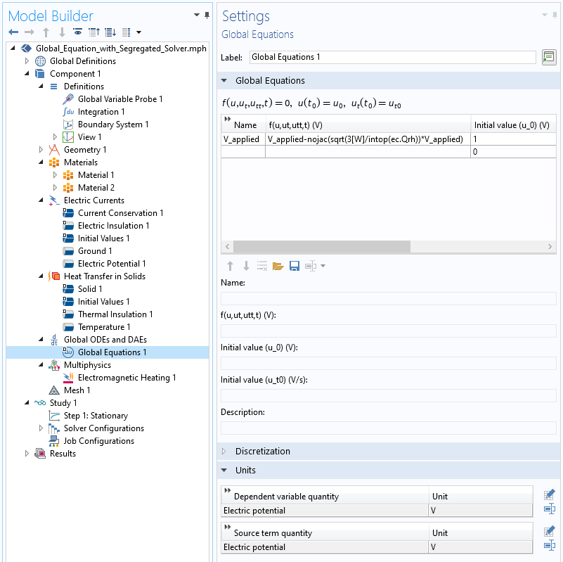
How to introduce an additional global equation to the model.

Let us support that what we would like to do is adjust the potential of one electrode relative to the other grounded electrode such that exactly 3 Watts is dissipated within the inclusion. The applied electric potential on the electrode is the variable V_applied, which we will control via the addition of a Global Equation into our model, as shown in the screenshot above. The equation that we enter appears quite simple:

V_applied-nojac(sqrt(3[W]/intop(ec.Qrh))*V_applied)

This equation, which will be solved for within each segregated iteration, will update V_applied. The applied voltage is scaled based upon the dissipation computed via an integration operator. The square root is used, since we know that, at least in a lumped model, losses are proportional to the square of the potential difference. Everything within the nojac() operator does not contribute to the Jacobian, and the terms within it are based upon the values at the previous segregated step, or the initial value if at the first step. Note that the initial value of V_applied must be nonzero, and a decent initial value will lead to faster convergence.

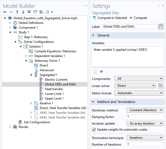
Segregated solver settings with the Global Equation solved after the Electric Potential.

Within the segregated solver settings, we do need to make sure that this segregated step is solved after the segregated step for the electric currents, since the update expression is based upon the computed electrical losses. We also want to make sure that the temperature fields are computed either prior to the electric currents or after the global equation is solved, since these can affect the loss computation when the material conductivities are nonlinear with temperature.

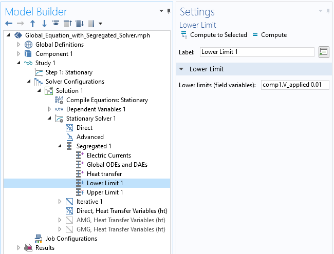
Upper and lower limits features in the segregated solver.

The segregated solver additionally gives us the option of providing both upper and lower limits to variables being solved for. That is, if any iteration would compute a V_applied that is larger, or smaller, than the specified values, the solver will simply use the limiting values instead. This is particularly helpful in terms of a lower limit, as we would never want the applied potential to go to zero, as further updates from that point would not be possible. An upper limit is also helpful if we know that there is some value above which the potential cannot be set.

As we solve this model using the segregated approach, we likely also want to monitor V_applied to see how it is being updated at each iteration. We can achieve this via a probe and via the settings shown in the screenshot below. The segregated solver also includes a Tolerance Factor, which multiplies the default tolerance of 0.001 as defined within the Stationary Solver feature. Making this number smaller than its default of 1 will tighten the convergence criterion of the solver. Note also that you can increase the number of iterations that the segregated solver takes if convergence is very slow.

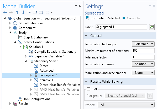
How to plot probes at every segregated iteration, as well as the tolerance factor setting.

For the problem that we have here, convergence is quite rapid. The convergence plot of the segregated solver, and the probe plot, are shown below. Of course, convergence for a nonlinear problem is never guaranteed, and this additional update of the global equation does typically slow convergence, but in a great many cases, this technique can be used robustly, especially when a reasonable initial value is chosen. It should be noted that, depending upon the physics and the value that you are controlling on, different forms of the update equation might be needed. In this case, we use a square root of a ratio, but you could also use a linear, or an exponential, scaling between iterations. We can also think of this approach as a kind of a proportional controller, or a fixed-point iteration scheme.

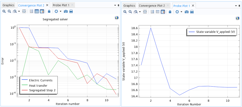
Convergence of the segregated solver, and the probe plot of the additional global equation.

The great advantage of this approach is that we get to our design point using just one solution, using the computationally efficient segregated approach. This one solution might take a few more iterations than without the global equation, but the advantage of getting to the desired solution quickly almost always outweighs this cost. Also, if you want to solve in the time domain, then this approach can be used without modification as long as the global equation can be satisfied at each time step.

There may be, of course, cases where this approach does fail, in which case you can employ an alternative method that uses a fully coupled, rather than a segregated approach, but that is a topic for an upcoming blog, so stay tuned!

Try It Yourself

The model file associated with this example is available via the button below: