

Proton therapy is a cutting-edge cancer treatment procedure whereby an energetic beam of protons is used to deliver ionizing radiation to the treatment area. The intensity, direction, and shape of the proton beam needs to be finely controlled to deliver the appropriate dosage to the tumor region while minimizing damage to adjacent healthy tissue. This blog post demonstrates how to model a pencil beam scanning nozzle to precisely steer the proton beam to the treatment field using the COMSOL Multiphysics® software.
The Advantages of Proton Therapy
Proton therapy, like other forms of radiotherapy, treats cancer by intentionally damaging the DNA of tumorous cells with ionizing radiation. This radiation damage interrupts their reproduction and ultimately eliminates the tumor cells. In proton therapy, the source of ionizing radiation is an energetic proton beam generated by a particle accelerator.
The key advantage to using a proton beam, instead of traditional X-rays, is its pronounced Bragg peak. With an X-ray beam, the delivered radiation dose is maximum near the shallow tissue region and falls off monotonically with tissue depth. This means that both shallow and deep healthy tissue will receive collateral irradiation during the course of treatment. In contrast, the proton delivers maximum dosage right before it comes to a stop, that is, near its maximum penetration distance. The shallow healthy tissue receives a comparatively lesser dose, while deeper tissues are spared entirely. By fine-tuning the energy of the proton beams used in the treatment plan, the medical physicist can ensure that the beams deliver an even dosage over the tumor region while sparing the adjacent healthy tissue.
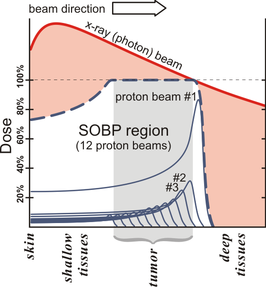 Dose versus penetration depth for a proton beam and an X-ray beam. Note the pronounced Bragg peak of the proton beam. Image licensed under GNU Free Documentation License, via Wikimedia Commons.
The transverse profile of the proton beam also needs to be controlled to match the shape of the tumor. The two most common methods are passive scattering and pencil beam scanning (PBS). Passive scattering makes use of one or more scattering foils to spread out the beam such that the target region (also known as the treatment field) receives nearly uniform irradiation. In contrast, pencil beam scanning, or spot scanning, divides the field into voxel-like subregions and treats each subregion with a narrow “pencil” beam.
Controlling the Proton Beam
The steering of the proton beam is controlled by the PBS nozzle system. At its simplest, the PBS nozzle consists of two dipole magnets aligned vertically and horizontally. The resulting uniform fields deflect the beam in the horizontal and vertical directions, respectively. By controlling the currents driving the magnets, the radiation technician can tune the magnetic field strength and thus control the extent of the beam deflection.
Numerical modeling of the PBS system is motivated by the rising interest in real-time treatment monitoring with magnetic resonance imaging (MRI), also known as MR-guided proton therapy. Since both the PBS nozzle and MRI system utilize strong magnetic fields, it is important that the mutual electromagnetic interaction between the two systems is thoroughly understood. This will determine any necessary intervention in order to maintain MR imaging quality as well as proton beam quality.
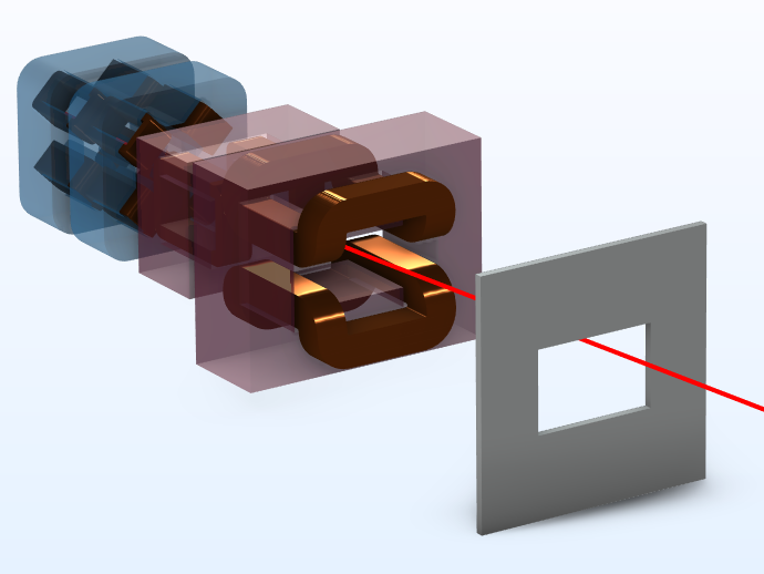 A 3D model of the pencil beam scanning nozzle.
Simulating the PBS
In this blog post, we will focus on the PBS system alone. The model consists of four separated function magnets — two dipoles and two quadrupoles (quads) — as well as a beam aperture and a target plane representing the treatment field.
 Part of the PBS model. The magnet system consists of two quadrupoles, labeled Q1 and Q2, a vertical scanning dipole (SV) and a horizontal scanning dipole (SH). Also depicted are a beam aperture and the target plane (location of treatment field).
The purpose of the quads is to shape the proton beam profile and ensure that it is matched to the upstream accelerator beamline (not modeled). The linear magnetic field gradient acts to focus the proton beam in one transverse direction and defocus it in another, hence the need for two quads. The strength of the focusing is controlled by the input quad currents.
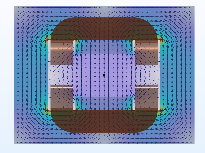
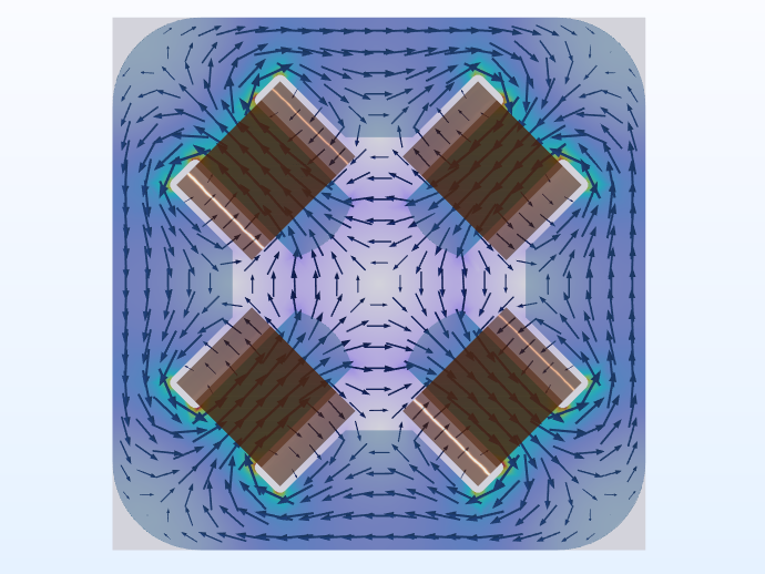 Magnetic field along the midpoint cross section of quadrupole 1 (Q1). Note the direction of the field arrows near the center. The Q1 field focuses the proton beam in the vertical direction and defocuses it in the horizontal direction. The other quadrupole (Q2) is rotated by 90 degrees and behaves in the opposite manner.
Downstream of the two quads are the two scanning dipoles. These magnets generate a constant uniform field within their pole gap in order to deflect the proton beam toward the desired target location. The magnitude of the horizontal/vertical deflection is determined by the magnetic field strength, which is in turn controlled by the input dipole currents. In the model, the user can specify the desired (x, y) target location in the treatment field, and the requisite coil currents are approximately calculated based on a fixed beam energy. For more fine-tune control over the beam target position, the user can adjust the coil currents directly.
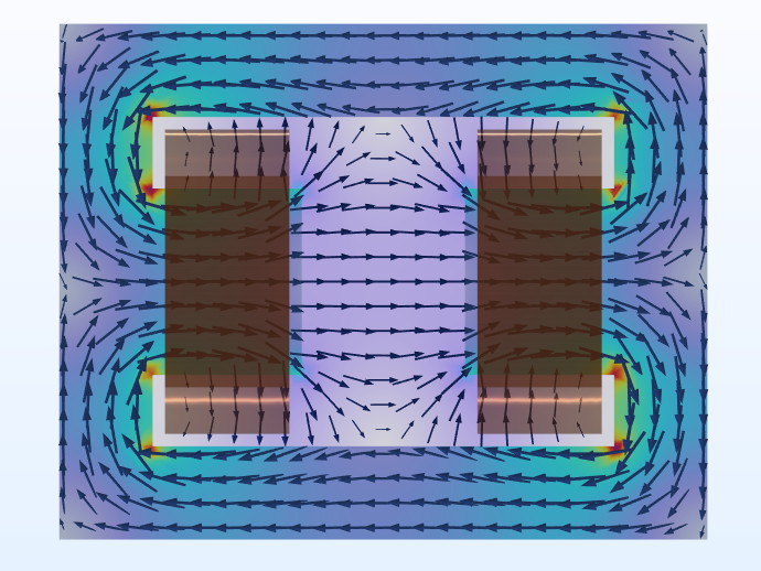
Magnetic field of the vertical scanning (SV) dipole on the left and the horizontal scanning (SH) dipole on the right.
Downstream of the two scanning dipoles are the beam aperture and the target isocenter. The beam aperture is the only part of the physical structure of the PBS nozzle that is modeled. The rest of the physical structure is omitted in this model for demonstration clarity but can be included in a comprehensive study.
To visualize the proton beam trajectory, the Charged Particle Tracing interface is used. The magnetic field distribution is incorporated seamlessly into the particle tracing simulation in order to accurately determine the path taken by the proton beam. (Note that scattering is omitted in this model for demonstration simplicity.) The proton beam typically varies across a wide range of kinetic energies in the MeV range, and this is taken into account as a model parameter.
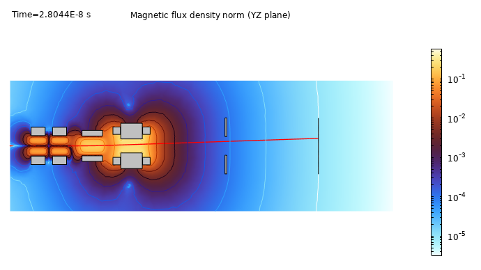
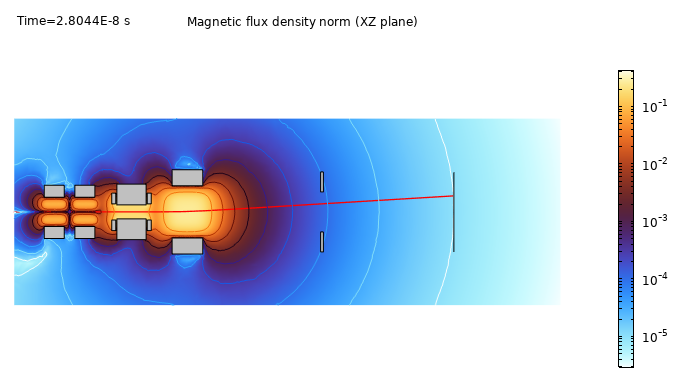
Plots of proton beam trajectory (red) and magnetic flux density norm along the yz- and xz-planes, respectively.
The figures above depict the proton beam and magnetic field configuration with the nominal beam positions set to x = 12 cm and y = 8 cm in the target plane.
Try it Yourself
Interested in trying out this multiphysics model for yourself? Click the button below to access the MPH file.
Further Reading
Learn about how simulation can advance other treatments in healthcare in these blog posts:


Comments (1)
Brian Sewart
February 12, 2026Great write up.