Using Differential Inductance and Coils in COMSOL Multiphysics^®

When modeling a low-frequency electromagnetic system involving coils, nonlinear materials, magnets, and moving parts, we are often interested in computing the differential inductance. Differential inductance quantifies the fields that arise in such electromagnetic systems when time-varying currents are driven through one of the coils. Differential inductances are especially useful for building simplified lumped models. Let’s cover some background on the theory and practice of using these differential inductances within the AC/DC Module, an add-on product to the COMSOL Multiphysics^® software.

A Brief Review of the Theory

The concept of inductance is relevant when there are one or more loops of wire along which current can flow. These loops, or coils, can be composed of one or many turns of wire. We will consider a source connected to one of the coils and refer to this as the primary. We will also consider a load connected to the other coils, referred to as the secondaries. These loads can represent an arbitrary combination of other electrical devices.

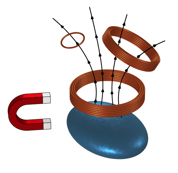
Several coils in space, with nonlinear magnetic materials and magnets nearby. Time-varying currents in one coil will induce fields in the other coils in proportion to the intercepted flux, which depends upon how the nonlinear magnetic materials are biased.

In the space around the coils, there can be nonlinear magnetic materials and magnets. The nonlinear magnetic materials can be driven into their nonlinear regime by the magnet, by current flowing through one of the coils, or both. Whenever a time-varying current is applied to the primary coil there will be an induced electromotive force — a voltage — on all coils, including the primary itself. Assuming that the frequencies of the applied signal are far below the resonant frequency of the system, it is sufficient to assume that this electromotive force will purely be due to the time-varying magnetic field. Under this assumption, the Coil feature is relevant.

Given a time-varying current flowing through one of the coils with index i, the electromotive force on any coil with index j, is proportional to the rate of change of flux linkage¹:

Applying the chain rule under the assumption that \Phi is solely a function of instantaneous current:

we see that the induced voltage is a product of L’_{ij} , the differential inductance with respect to current, and \dot{I_i}, the rate of change of the applied current. Note that if all materials in the system are linear, if no magnets are present, and if we neglect inductive losses in conductors, then we can simplify to:

 
where L_{ij} is the secant inductance and is computed by default whenever a Coil feature is used. On the other hand, computing the differential inductance takes some extra steps.

To understand how the differential inductance is computed, we first need to turn our attention to the flux linkage, which is commonly described in introductory engineering textbooks as the integral of \mathbf{B}_i, the magnetic flux due to the excitation of coil i passing through the surface, S_j, bounded by a thin loop of wire representing coil j:

However, as we can see from the image above, most coils will have significant cross-sectional area, so it is not possible to simply define a surface, S_j. Instead, we apply the divergence theorem and the fact that \mathbf{B=\nabla \times A }, and compute \Phi as the volume integral of the magnetic vector potential, \mathbf{ A } dotted with the direction that current can flow in the coil, \mathbf{ J }:

This quantity is automatically computed by the software whenever using the Coil feature and is referred to as the coil concatenated flux.

This concatenated flux can be a function of many different variables, although earlier we assumed that it was solely a function of the instantaneous current. Let’s now look at how to compute the derivative to extract the differential inductance.

Computing Differential Inductance

To compute the differential inductance, we need to evaluate the derivative of the coil concatenated flux in all coils with respect to the applied current in the primary. This can be done with the Sensitivity interface, which we’ve previously covered in our blog post “Computing Design Sensitivities in COMSOL Multiphysics^®” and will briefly review. The usage of this interface begins with defining a Global Objective feature, where we enter the expression for the coil concatenated flux. We also need to define at least one Global Control Variable, which is a variable used for taking the differential of the objective. Here, we enter a variable name that multiplies the DC current flowing through the primary. With this setup, the Sensitivity study step can be combined with an Auxiliary Sweep over the applied current, and the differential inductance over a range of applied currents can be computed.

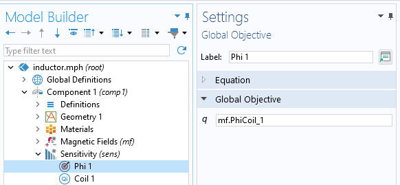
Defining the objective function within the Sensitivity interface.

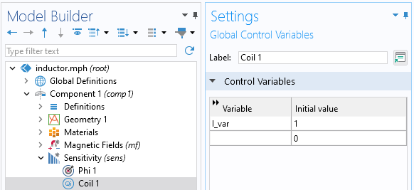
Defining the control variable within the Sensitivity interface.

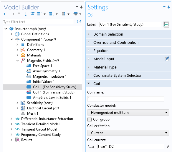
Using the control variable within the Coil feature to set up a differentiation with respect to the current.

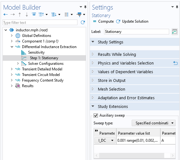
Sweeping over a range of currents in combination with computing the sensitivities.

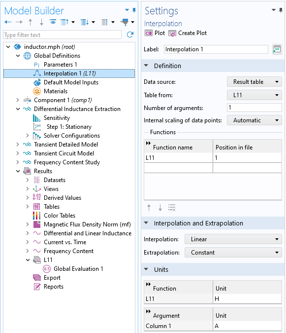
After solving, create an Interpolation function that refers to an Evaluation Group so that the results of the differential inductance calculation can be used elsewhere in the model.

With these fundamentals of the theory and workflow in mind, let’s now look at a few examples.

A Nonlinear Inductor

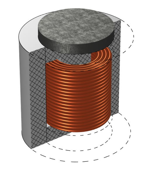
To start, we will model a coil inside a core made of an alloy powder core ferrite, a nonlinear magnetic material that has very low loss. We will treat the model as 2D axisymmetric. The coil is composed of 80 turns of 1 mm diameter wire and is operating at 50 Hz, so there will be negligible skin effect in these wires. Thus, the AC resistance of the coil is quite accurately predicted by the DC resistance. In this situation, we can use the Multiturn Coil Domain feature. We can solve this model in the time domain and get the nonsinusoidal current through the inductor in response to a sinusoidal applied voltage.

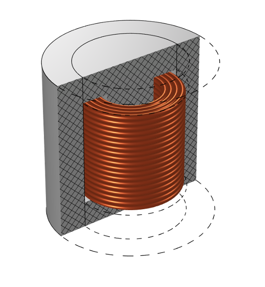
An inductor composed of coil around a BH nonlinear core.

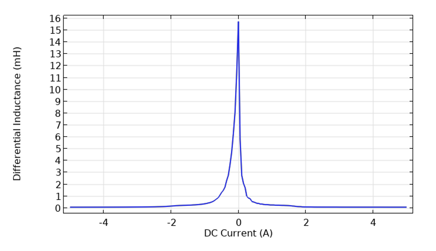
We first solve this model over a range of DC currents to get the differential inductance, as plotted below, along with the secant inductance for comparison.

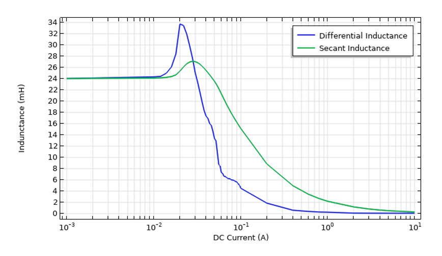
Differential and secant inductance of the inductor with a nonlinear magnetic core material over a range of applied DC currents.

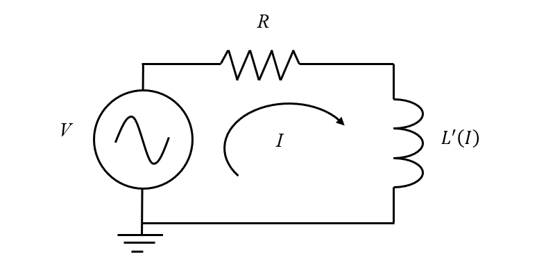
The equivalent electrical circuit model of the nonlinear inductor with the differential inductance as a function of current.

Now that we have this differential inductance, we can use it within an electrical circuit model to quickly predict the transient behavior. Our electrical circuit model needs only three features, in addition to the default Ground Node feature:

• Resistor feature
• Inductor feature
• Voltage Source feature

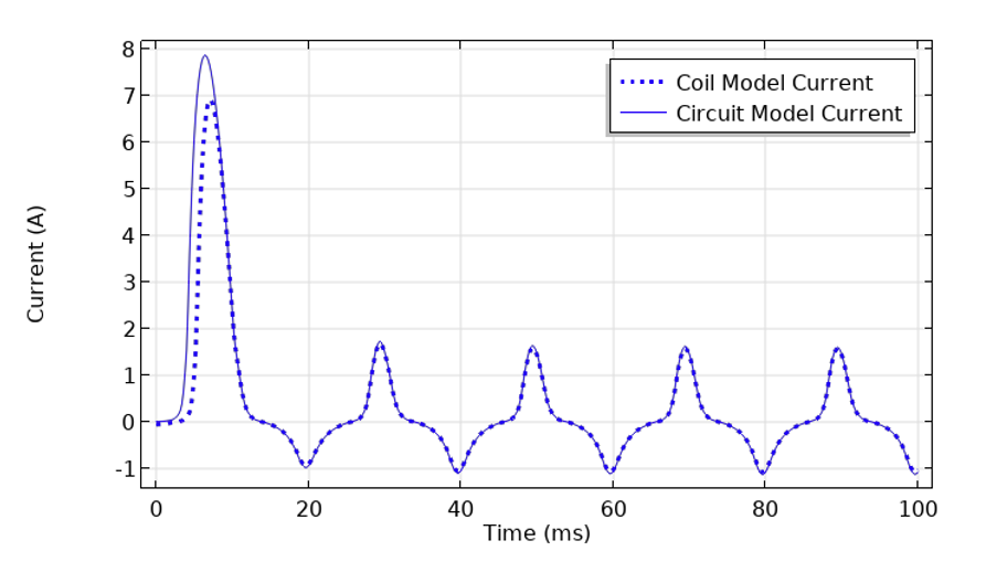
We use a Resistor feature with resistance equal to the computed Coil resistance. In series with that, we add an Inductor feature with a nonlinear inductance defined via the Interpolation table that stores our previously computed differential inductance. This nonlinear inductance can be made a function of the absolute value of the current, since the nonlinear behavior is not dependent upon the sign of the current. Finally, the Voltage Source feature, can be placed in series. Together, these three features create a lumped model that can predict the response. The results from this lumped model can be compared to the finite element model. Note that over the first few periods, the models are still only starting to approach the periodic steady-state response of this nonlinear system.

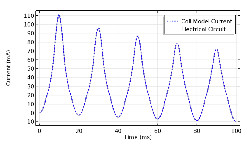
Plot of the current through the inductor with an AC voltage source applied. Results of the electrical circuit and magnetic fields models agree.

These time domain data can also be Fourier transformed into the frequency domain, which more clearly identifies the higher harmonics that are introduced by the material nonlinearity. Since the electrical circuit model is quick to solve, we can also quickly examine a wide range of operating conditions. As expected, there is more high frequency content as the device is driven into the nonlinear regime.

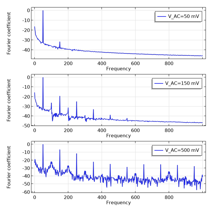
Plot of the frequency content of the current, with increasing peak-to-peak voltage.

A Nonlinear Inductor Biased with a Magnet

For illustrative purposes, we will now modify the above example with a magnet placed next to the core. This magnet will contribute to the coil concatenated flux and will bias the nonlinear material. The differential inductance is now dependent upon both magnitude and sign of the applied current. It is important to note that the secant inductance contains the contribution of the magnet itself to the concatenated flux, but this time-invariant flux does not contribute to the back-induced voltage. The magnet only acts to alter the B-H relationship of any nonlinear materials that are present. That is, a magnet will not affect the response of an inductor made only of linear materials. However, it is important to keep in mind that a magnet will always introduce a bias into the secant inductance. Therefore, whenever a magnet is present in your model, it is always best to work with the differential inductance even if all materials are linear.

A magnet placed on top of the B-H nonlinear core will bias the response.

The differential inductance is nonsymmetric with respect to the sign of the DC current for this biased inductor.

This differential inductance can again be used within an electrical circuit model, and again we see that results agree very well except for during the startup period. This disagreement over the startup period highlights the difference between the model that computes the spatially varying fields and spatial evolution of the saturation of core, as compared to the lumped model.

Agreement between the spatial finite element model and the lumped circuit model with the biased differential inductance.

The Nonlinear Response of a Transformer

Next, let’s look at a transformer composed of two identical coils wound around a core made of alloy powder core ferrite. Symmetry can be exploited not only to reduce the model size, but also to reduce the amount of data that needs to be computed, since L’_{11} = L’_{22} and L’_{12} = L’_{21}. Although, in the general case, the differential inductances can be a function of both I_1, the current in the primary, and I_2, the current in the secondary, for this symmetric structure L'(I_1,I_2) = L'(|I_1+I_2|,0). That is, we only need to compute the differential inductances L’_{11} and L’_{12}; over a range of I_1, while holding I_2=0, rather than sweeping over two variables.

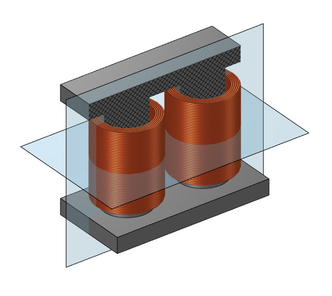
A transformer composed of two identical coils wound around a symmetric core. The two planes of symmetry are visualized.

Once these two differential inductances are computed, a set of functions is used to define all four terms of the mutual inductance matrix. These terms can be used within an electrical circuit model of the same transformer. Due to the nonlinearity, the coupling between the two coils is modeled with a Current-Controlled Voltage Source feature, as illustrated in the figure below.

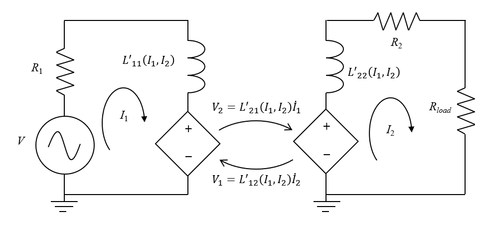
The equivalent circuit of a transformer with a nonlinear core material.

Solving for the response of this transformer using the full three-dimensional model has a significant computational cost, while solving for the electrical circuit model is very quick. The results again agree very well, although it is important that the differential inductance matrix be computed over all possible operating conditions. This one-time cost for computing the differential inductance matrix can be parallelized via a batch sweep or cluster sweep to exploit all your available computational resources.

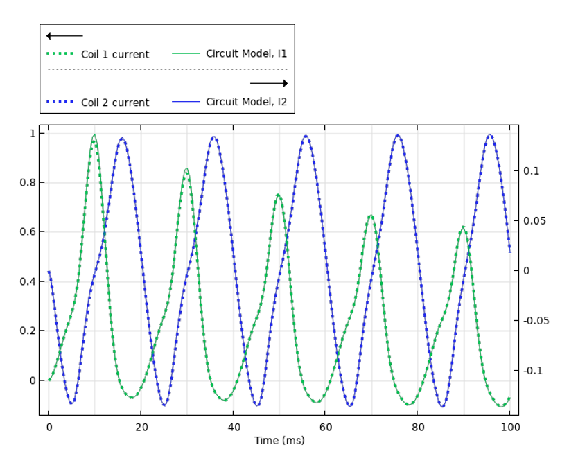
A sinusoidal AC voltage imposed on the primary leads to a nonlinear current through the primary and secondary. The voltage on the primary and current on the secondary are compared between the full model and the electrical circuit model.

The Dynamic Response of a Solenoid

Now let’s look at a solenoid composed of a coil inside an iron housing with an iron plunger. The plunger is mounted such that it can only move along its axis. We will assume that the permeability of the iron is constant over the range of expected fields and will neglect material nonlinearities. We will also assume that the housing and plunger are composed of parts that are bonded together with an insulating material, thereby minimizing any induced currents circulating about the axis, and will therefore treat the iron as lossless.

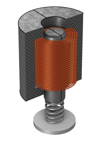
A solenoid consisting of a coil inside an iron housing with an iron plunger held in position by a spring.

A spring holds the plunger in its equilibrium position outside of the housing. When a voltage is applied to the coil, current starts to flow and forces the plunger towards the center. In this situation, there is no material nonlinearity, so the concatenated flux is linearly dependent upon the time-varying current, I, but changes nonlinearly with u, the plunger z-position:

So, via the chain rule, the back-induced voltage is:

The first term accounts for the fact that the secant inductance varies as the plunger changes position. The second term introduces an additional back-induced voltage when the plunger is moving at velocity \dot{u} through a nonzero magnetic field.

Keeping in mind that concatenated flux is linear with applied DC current, I_{DC}, and differentiating the first equation with respect to position when a DC current is applied, we see that:

So, to compute the derivative with respect to position, we use the Sensitivity interface in conjunction with the Moving Mesh interface to compute the partial derivative of the concatenated flux with respect to an infinitesimal change, \delta, in z-position at a fixed DC current:

We use the Moving Mesh to introduce both a finite and an infinitesimal change in the z-position and take the partial derivative only with respect to the infinitesimal displacement, \delta, while sweeping over a range of different positions, u, along the plunger stroke. This partial derivative now gives us the ability to build a simple electromechanical lumped model that couples the circuit model to an equation of motion of the plunger.

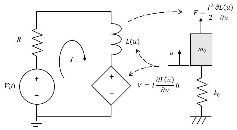
The electromechanical lumped model consists of a circuit model and a lumped mechanical model coupled by the force, the position-dependent secant inductance, and the back-induced voltage when the plunger is moving.

As we can see from the sketch of the lumped system, the electrical system couples to the mechanical system via the force. To understand how we arrive at the expression for force, let’s look at the expression for the total magnetic energy in the system, which varies with current and plunger position:

The total force on the plunger can be found via the method of virtual work, where, in the case of linear magnetic materials, the force in the axial direction is given by taking the partial derivative of the total magnetic energy with respect to an infinitesimal displacement:

That is, the force is a function of the current through the coil and the partial derivative of inductance with respect to position, which we already computed. So, along with our model of the solenoid, we also simultaneously solve the ordinary differential equation for the position of the plunger:

where u_0 is the equilibrium position of the plunger. This equation can be solved via a separate Global ODEs and DAEs interface or via a Global Equations feature that can be added to any physics interface. So, this equation can be used to solve for the motion in conjunction with solving for the Magnetic Fields interface, and it can be solved in conjunction with the Electrical Circuit interface.

We will let the plunger oscillate freely along the axis and examine the results in terms of a set of inputs that produce some interesting dynamics for the purposes of illustrating that the lumped model agrees very well with the spatial model used to compute the lumped parameters.

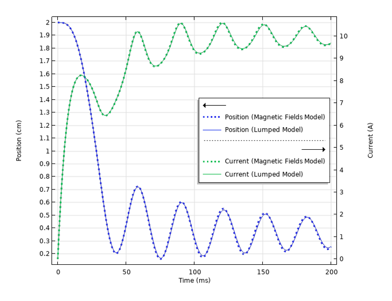
Comparison between the detailed model of the magnetic fields of the solenoid and the lumped model.

Building Your Own Lumped Models

We have looked here at a set of four examples highlighting the capabilities of the COMSOL Multiphysics^® software to extract not just the differential inductance, but the derivative of the coil concatenated flux with respect to other input variables. The resultant quantities can be used to build lightweight lumped models that can be good predictors of system performance.

Are you wanting to extract differential inductances and build these types of lumped models? Download these examples from the Application Gallery:

Reference

1. 1. D. Cheng, “Field and Wave Electromagnetics”, 2nd ed., Addison-Wesley, 1991