

In microfluidic systems, fluid flow is always laminar. This is both a benefit and a burden — a benefit because the flow field is stationary, and a burden because species mixing occurs primarily by diffusion, which can be time-consuming. A simple way to mix chemical species in a microfluidic chip is to use a serpentine channel structure. Using the COMSOL Multiphysics® software, the periodicity of such a structure can be exploited to determine the required channel length that will ensure that the chemical species leaves the system well mixed.
Modeling Periodic Microfluidic Systems Using COMSOL Multiphysics®
An example of a microfluidic device featuring serpentine channels is shown in the image below. Diluted solutions of chemical species can enter the system via the two inlets. The fluids come together and flow through the serpentine channels. The mixing of the chemical species occurs by diffusion, as the flow in microfluidic systems is laminar. For setting up an efficient simulation, we can exploit the periodic structure and consider a single repeating unit cell.
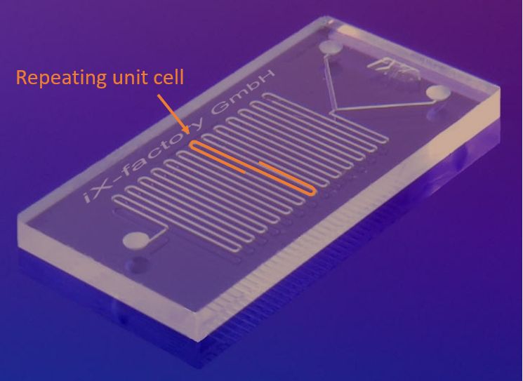
A typical microfluidic device. Image was modified. Original image by IX-factory STK — Own work, licensed under CC BY-SA 3.0, via Wikimedia Commons. The original work has been modified.
The serpentine channel featured here was also discussed in two previous blog posts. In the approach discussed in the first of these blog posts, “Using General Extrusion Operators to Model Periodic Structures”, the laminar flow is solved for one repeating unit cell, reducing the computational load. The velocity field is then mapped onto the full geometry containing multiple repeating unit cells using a General Extrusion operator. Using the mapped velocity field, transport of diluted species is solved on the full geometry, as shown in the following figure.
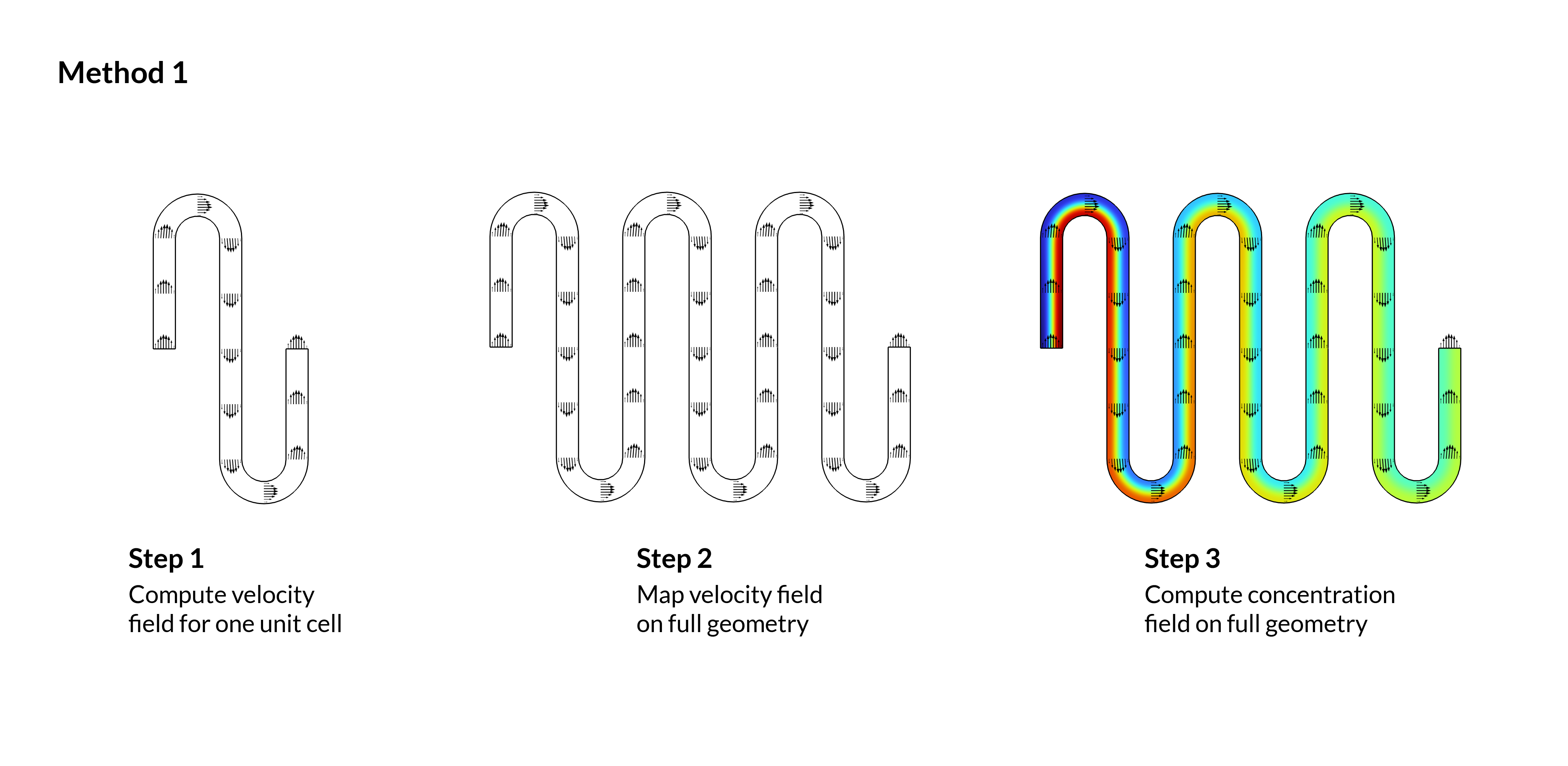
The first modeling approach for simulating a periodic microfluidic device. The velocity field is simulated in one unit cell and is mapped onto the full geometry. The concentration profile is computed on the entire geometry.
In the second blog post, “Exploiting Periodicity in Models with High Péclet Numbers”, the model is further simplified. The focus is on microfluidic systems that have a high Péclet number. The species transport is dominated by advection rather than diffusion, and consequently, the downstream solution does not affect the upstream solution. Therefore, it’s not necessary to compute the species transport on the entire device, as is done in the first approach.
Thus, for high Péclet numbers, the species transport can be computed sequentially, one unit cell after the other. To do so, the velocity field is solved on one unit cell, as shown in the image below (“method 2”). Then, the concentration field is solved in a unit cell. Using the General Extrusion feature, the concentration field at the outlet is mapped back to the inlet. To ensure that the previous solution is used for the concentration mapping in the next iteration, the Boundary ODEs and DAEs interface and the Previous Solution feature are used.
In this blog post, we introduce a different route to achieving the same goal: transferring the results from the outlet back to the inlet for the sequential computation of the species transport. Instead of a boundary ODE, we use a state variable. The state variable is easier to implement than the ODE. This reduces the complexity of the model.
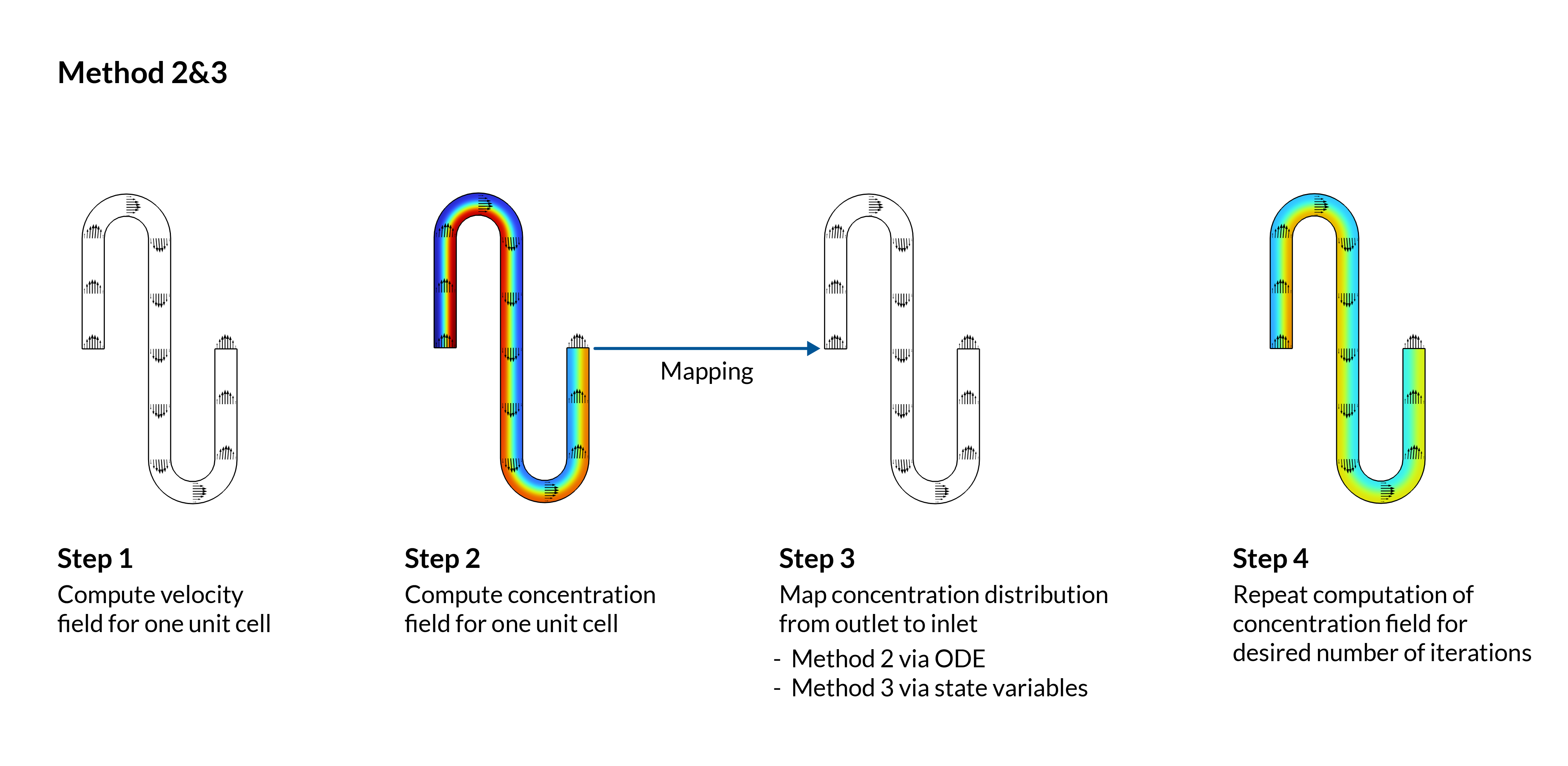
The second and third modeling approaches for simulating a periodic microfluidic device using only a single unit cell. The methods differ in step 3. The mapping of the concentration profile from the outlet to the next unit cell inlet can be implemented either using an ODE or a state variable. (The latter approach is explained below.)
General Extrusion and a State Variable
The modeling begins with the definition of the General Extrusion operator, genext1. The operator can be found under Definition > Nonlocal Couplings. The operator is defined on the boundary of the outlet. It maps an expression — in this case, the concentration — from the outlet to the inlet due to the specified displacement in x.
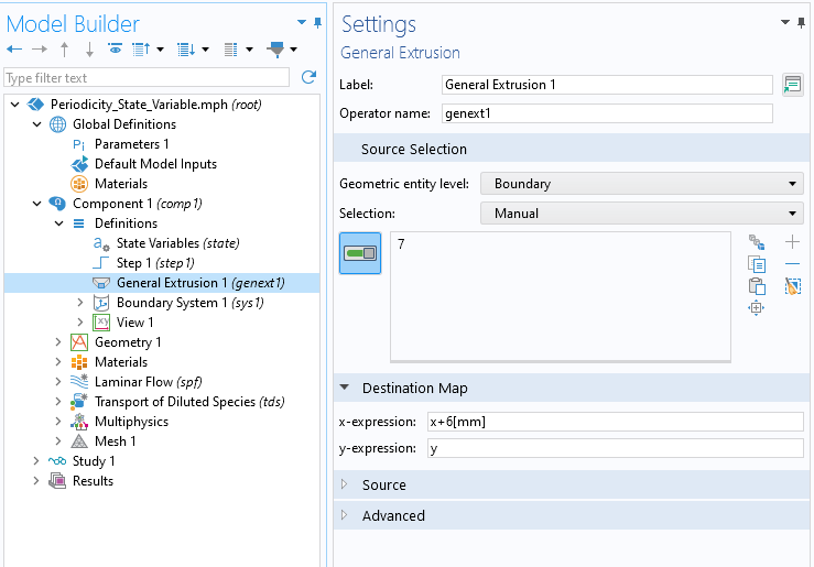
The General Extrusion operator maps a variable from one boundary to another by an offset of 6 mm in the x direction.
In the second step, the state variable is defined on the boundary of the inlet. The State Variables feature can be found under Definitions > Variable Utilities. State variables are treated as dependent variables in the model. In contrast to the usual dependent variables in a physics interface, state variables can be set to be updated before or after each converged parameter step or time step, or only at initialization. The settings for the state variable are shown in the screenshot below. The state variable is called c_b, and a step function is used as an initial value to display the initial concentration gradient at the inlet. The step function is located at x = 0.5 mm, and the initial concentration varies from 0 to 1 mol/m3 depending on the x-location. The state variable is always updated at the beginning of a parameter step. This means that the concentration at the outlet from the previous step is mapped onto the inlet for the next iteration.
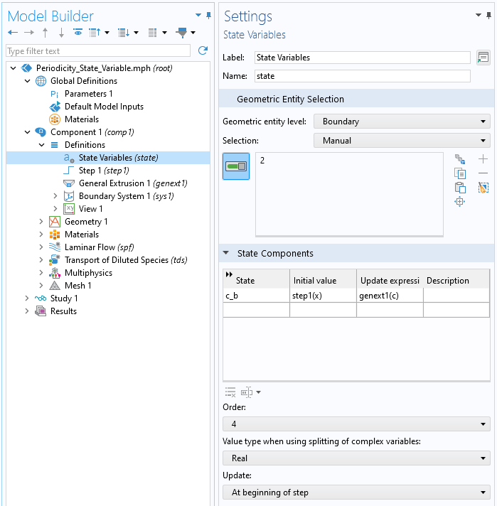
The Settings window for the state variable.
The state variable c_b is used as the concentration at the Inflow boundary in the Transport of Diluted Species interface. The data of the state variables is stored at Gauss points, not at node points. Because of this, we select Flux (Danckwerts) for Boundary Condition Type, instead of Concentration constraint. The concentration condition is applied to the node points, while the Danckwerts condition imposes a flux at the Gauss points.
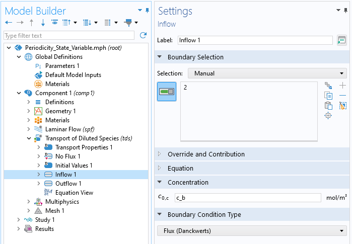
The state variable c_b is set as the concentration at the inflow boundary.
To minimize an extrapolation error, the Identical Mesh feature is used at the inlet and outlet boundaries.
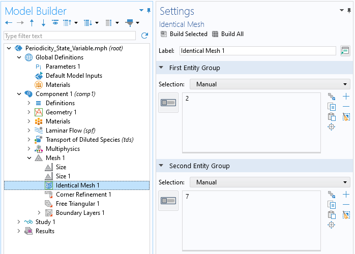
The Settings window for the Identical Mesh feature. Boundaries 2 and 7 are the inlet and outlet boundary, respectively.
Similar to the previous blog post, we compute the model in two steps. The study step settings are shown in the image below. In the first study step, only the Laminar Flow interface is computed for one unit cell. The flow field is the same no matter how many repetitions of the unit cell are considered. This is not the case for the species transport. In the second step, Transport of Diluted Species and State Variable are computed. Additionally, we introduce a parameter n_unit_cells for the sequential computation of the repeating unit cells. This parameter is used in the auxiliary sweep and is swept from 1 in increments of 1 to the maximum number of unit cells, which is 15 in this case. At the end of each computation, the state variable is updated and the concentration field of the outlet is mapped onto the inlet for the subsequent unit cell. The Run continuation for setting is set to No parameter, and Reuse solution from previous step is set to Yes in order to update the state variable correctly.
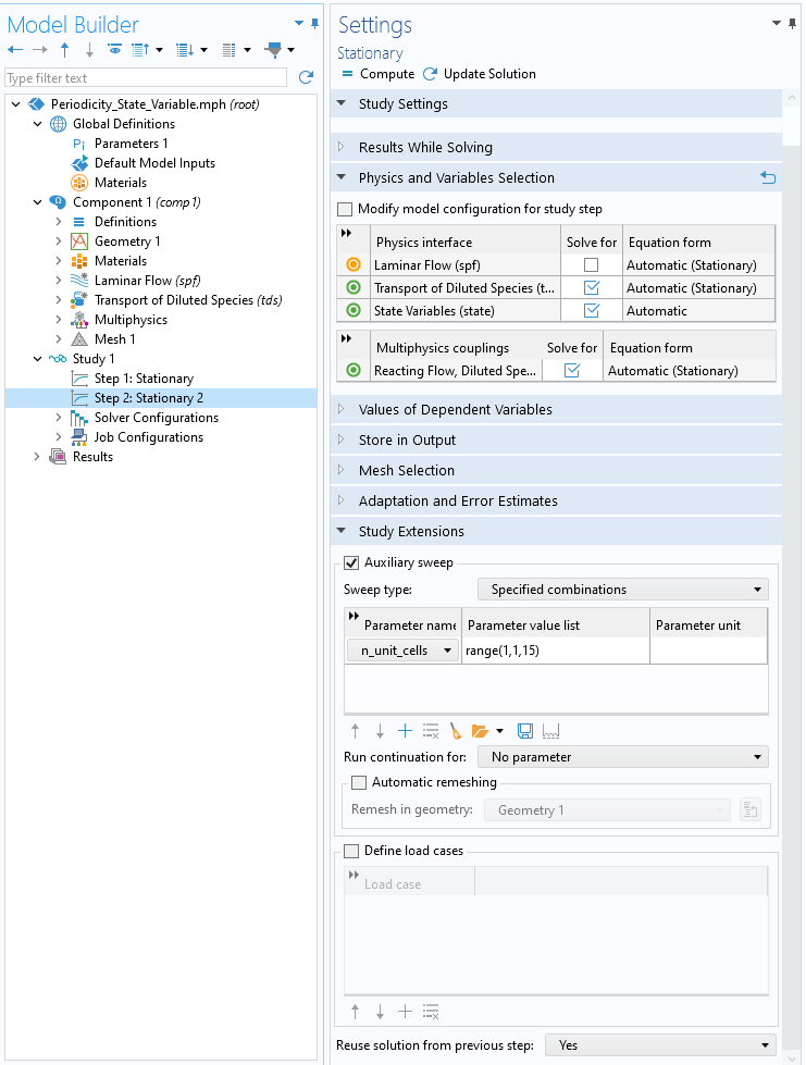
The study step settings, with the Auxiliary Sweep feature enabled. The parameter n_unit_cells reflects the number of unit cells.
As a result, we get the concentration profile over all repetitions of the unit cells. In the following figure, the first three unit cells are shown.
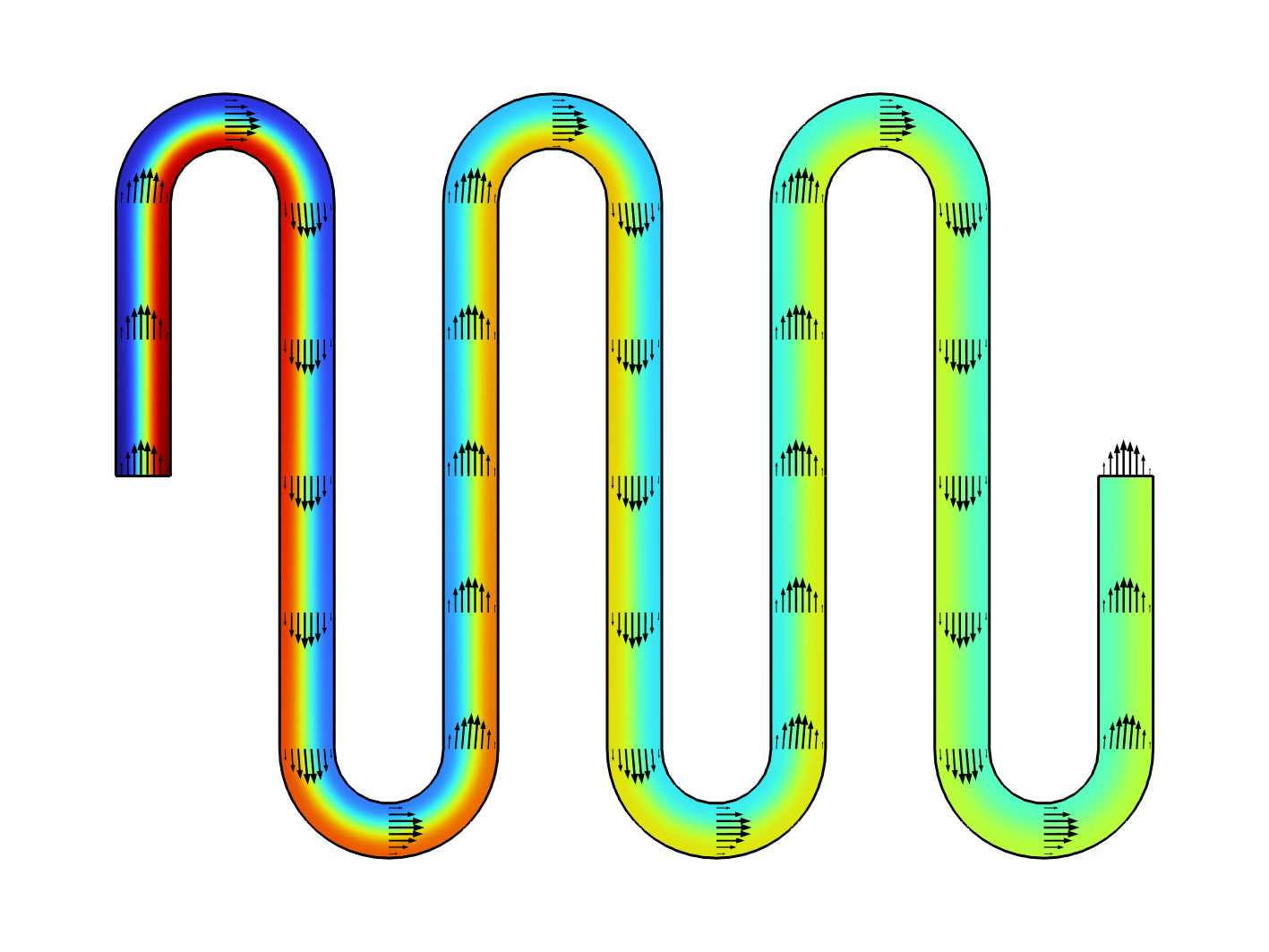
Concentration profile of the first three unit cells.
The simulation results presented here can be used to determine the degree of mixing and the needed channel length. The efficient approach of using the auxiliary sweep enables us to scale up the mixer to our heart’s content. To further measure how well a system is mixed, we can consider the mixing index (MI). The mixing index is computed across the channel cross section and is defined as follows:
where \textless{c}\textgreater displays the average concentration across the outlet boundary and {\sigma} is its standard deviation.
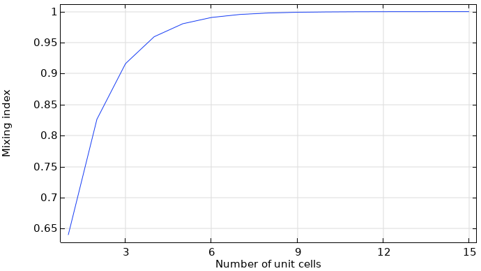
The mixing index as a function of the number of unit cells.
The plot shows the mixing index at the outlet of each unit cell for 15 repetitions. A mixing index of 0.98 is already reached after 5 unit cells.
Key Takeaways
The method shown here is very similar to that discussed in our blog post “Exploiting Periodicity in Models with High Péclet Numbers” . These methods simplify the model and save computational resources. The main difference to the previous method is that instead of an ODE, a state variable is used to save and transfer the outlet concentration to the next iteration. The method using the state variable is easier to implement since it doesn’t require any changes in the solver configurations. Therefore, we recommend using the state variable method to model systems with a high Péclet number. This approach can also be applied to more complex applications, such as the mixing of several chemical species that react to other species.
Further Learning
Want to learn more about some of the features mentioned here? Then check out these blog posts:
- Get an in-depth look at working with Gauss points: “Introduction to Numerical Integration and Gauss Points”
- Learn more about the functionality of the State Variables feature: “How to Use State Variables in COMSOL Multiphysics®”
- See how to use the General Extrusion operator: “Mapping Variables with General Extrusion Operators”
- Learn more about the usage of the General Extrusion operator: “Examples of the General Extrusion Operator”

Comments (0)