Accelerating Model Convergence with Symbolic Differentiation

Did you know that the COMSOL Multiphysics® software includes a symbolic differentiation engine that is automatically used whenever you set up and solve a nonlinear problem? This feature ensures high robustness of the software when solving such models, but it does come with some costs. Today, we will look at this capability in a few different examples and examine its benefits and tradeoffs.

Solving a Simple Nonlinear Problem with Symbolic Differentiation

Let’s start by looking at a relatively simple, single degree of freedom, nonlinear problem — the implicit equation:

We can say that T represents a lumped temperature of a system; Q represents a heat load; and the denominator of the above equation, (1+T^2/100), represents a system thermal conductance.

We want to solve for different values of the parameter Q. The solution to such a nonlinear problem can be found via the damped Newton’s method, which can be done in COMSOL Multiphysics by writing out the residual:

and then entering it into the Global Equation interface, as shown in the screenshot below.

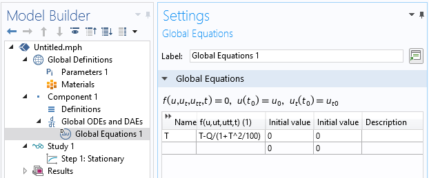
The Global Equation interface, used to solve our nonlinear equation.

We can solve this equation for a range of different values of Q and plot the solution, as shown below.

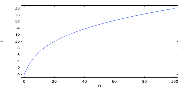
Solution to a single degree of freedom nonlinear problem.

For illustrative purposes, let’s plot out the residual for a range of values of T, and for select values of Q, in the plots below. The dots at the zero crossing are the solution from the above plot.

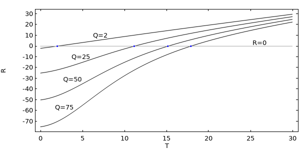
Plot of the residual for different values of the parameter Q. The value of T from the zero crossing is the solution to the nonlinear equation.

Let’s also plot out the corresponding derivative of the residual (the Jacobian) for the same range of T and values of Q below.

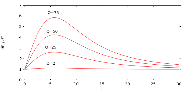
Plot of the derivative of the residual for different values of Q.

We see that, for increasing values of Q, the Jacobian is a more nonlinear function. We can also (for this simple case) manually write out the derivative:

Keep in mind that the software is automatically able to take this derivative via symbolic differentiation and use it within the Newton steps.

Now, it is the denominator of the second part of the residual that makes this expression a bit complicated (recall that this term can be thought of as the thermal resistance of the system). It turns out that we can ignore this term, if we want, by wrapping the nojac() operator about the term in the denominator:

R(T) =(T – Q/nojac(1+T^2/100))

and modifying the Global Equation, as shown in the screenshot below.

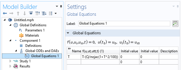
Screenshot showing how to use the nojac() operator.

As a result, everything within the nojac() operator will be ignored by the symbolic differentiation engine. That is, the terms within this operator have no contribution to the Jacobian. The derivative of the residual with respect to T is now simply:

We can see by examination that this simplified derivative is only a good approximation for low values of Q, and the effect is that the solver is not able to converge to the solution for all values of Q. So, we have made the problem a bit simpler by avoiding the (in this case very small) overhead of taking the derivative of some terms, but we have made it unsolvable in some cases.

Using the nojac() Operator in COMSOL Multiphysics®

Let’s also consider a couple of other ways in which we could use the nojac() operator.

If we were to write our global equation as:

R(T) = nojac(T – Q/(1+T^2/100))

Then the derivative will be exactly zero, and this problem cannot be solved at all, so this case isn’t interesting.

Let’s also try applying nojac() to just one term:

R(T) = T – Q/(1+nojac(T)*T/100)

Now, our derivative is:

This is very close to the exact residual, and, at least in this case, the solver will converge for all values of Q, even with this approximation of the Jacobian. Although the computational cost hasn’t gone down, the notable point here is that we can apply the nojac() operator to any subset of the terms for our residual.

So, what have we learned so far?

1. You can use the nojac() operator to omit terms from contribution to the Jacobian
2. Omitting terms will have an effect upon the convergence of the nonlinear solver
3. Omitting terms reduces the size of the computational model

The last point, though, is not all that apparent on this small example.

Reducing the Size of a Large Nonlinear Model

Let’s look now at a larger model in three dimensions. We solve a heat transfer problem on a 1-cm cube and apply an Extremely Fine mesh on this part, giving us a larger model; about 3 million degrees of freedom.

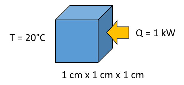
Schematic of a simple heat transfer problem to investigate with an extremely fine mesh.

We also make the material properties a function of temperature, and using a material property similar to what we’ve already seen, we define the material thermal conductivity via the user-defined expression:

(1+(T[1/K])^2/100)[W/m/K]

This is done directly within the physics interface, as shown in the screenshot below.

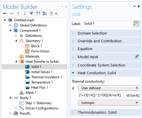
The thermal conductivity manually defined as a function of temperature.

When we solve this problem using all of the default settings, the model will need four iterations of the damped Newton method to solve, take about 135 seconds of wall-clock time, and use a bit over 12 GB of memory on a typical desktop computer. During the solution process, we also get a message in the log that says:

Nonsymmetric matrix found.

This message is a consequence of the temperature-dependent terms in the material properties. That is, the nonlinear terms within the material property make the Jacobian matrix nonsymmetric, and the model will as a consequence take more memory to solve. Let’s now wrap the entire material property expression in the nojac() operator:

nojac(1+(T[1/K])^2/100)[W/m/K]

Rerunning the model, we see that the model does still converge and takes about 10 GB to solve, but now takes five iterations of the default damped Newton method. That is, memory requirements have gone down, but the number of iterations to convergence has gone up. Most interestingly, the wall-clock solution time is 125 seconds, a bit less than before! Why is this? The solver needs more iterations to converge, but each iteration takes less time, since the Jacobian matrix is symmetric and less data needs to be worked with.

So, in this case, using the nojac() operator reduces both the wall-clock solution time and reduces the memory needed, despite the fact that more iterations are needed to converge to the solution! Also note that we converge to the same solution, since the material properties themselves are still correctly evaluated, using the updated material property expression.

Avoiding Nonlocal Coupling Terms

Let’s finish up with one more example: the crushing of a thin-walled container containing a compressible gas, as shown in the figure below. This can be modeled with the Shell formulation available within the Structural Mechanics Module.

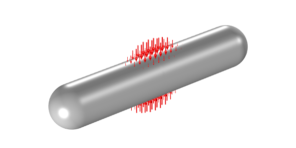
A thin-walled tank containing compressible gas with an applied external crushing load.

By exploiting symmetry, we can reduce our model to 1/8 of the full model. We apply a distributed load that approximates the crushing, as well as a pressure load representing the internal compressible gas. To represent the compressible gas, we use the approach of computing the volume of the deformed container, similar to what is done in our example of the compression of an air-filled hyperelastic seal. That is, by using an integration coupling operator, we apply a uniform pressure load over the entire surface of the tank, and this pressure is computed based upon the deformation of the entire tank.

The effect of this nonlocal coupling is that the deformation of every part of the tank affects the pressure, and the pressure affects the deformation everywhere, so our Jacobian matrix becomes quite dense. When this is solved using the default Extremely Fine mesh setting, the model takes about 12 GB of memory and 400 seconds to solve this ~22,000 degree of freedom model.

Screenshot showing the modified pressure within a model of a crushed tank.

However, simply by wrapping the nojac() operator about our applied pressure, we omit the nonlocal coupling and the memory requirements and solution time go down. This way, we need only 3 GB of memory and 10 seconds to converge to the same solution!

Concluding Thoughts

By default, the software will always take the exact Jacobian, since this gives us the greatest possibility of convergence. In general, we would rather sacrifice some time and memory to get a solution as robustly as possible. However, we see that we do have the ability and flexibility to omit selected terms from the Jacobian matrix. If we want to use this capability, we have to explicitly modify material properties, modify the underlying governing equations, or write our own variable expressions within the model, so this is a bit of an advanced user feature.

Of course, using this functionality will approximate the Jacobian, and this will sometimes slow down, or even prevent, convergence, so don’t use it in those cases. However, if the model does converge with the nojac() operator being used, then it will still converge to the same solution as with the full Jacobian evaluation, and may use less time and memory, so it is a good feature to be aware of as you build complex multiphysics models.