Computing Transformer Equivalent Circuit Parameters

Transformers are ubiquitous to the electrical industry. Whether it’s power transmission and distribution, heavy industries, instrumentation, electrical vehicles, or consumer electronics, transformers of all shapes and sizes are an integral part of the systems. There are different types of transformers: power transformers shift power from one electrical system to another at different voltage levels, instrument transformers are used for voltage and current measurements, isolation transformers couple signals between two circuits with galvanic isolation, high-voltage transformers are used for generating voltages of the order of kV or higher, and so on. The equivalent circuit parameters of a transformer determine its performance and therefore become crucial for its design and development.

In our recent blog post “Extracting Electrical Circuits from Electromagnetic Simulations”, we explain how you can extract equivalent RLC networks from any electromagnetic model, which is also applicable to any transformer with concentrated windings. In this blog post, we will show an example of a high-frequency ferrite core transformer with primary and secondary coils consisting of multiple sections, as well as provide an overview of circuit parameters and analyses.

Introduction

There are various factors that play an important role in determining the performance of transformers. The equivalent impedance of a power transformer affects the short circuit or fault levels. Magnetizing inductances determine the inrush currents in large transformers, whereas leakage inductances play a decisive role in choosing the switching frequencies of power electronic circuits. Parasitic capacitances become significant in the working of high-frequency transformers. The behavior of transformers is largely characterized by their equivalent lumped electrical circuit parameters. Therefore, using simulation to extract the equivalent circuit parameters of a transformer is invaluable to the design process.

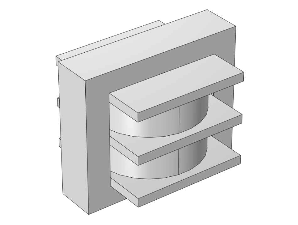
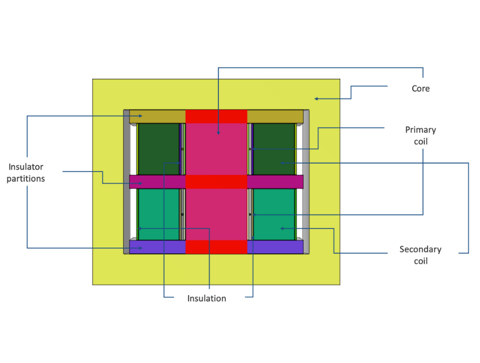
Left: A transformer geometry model. Right: A sectional view of the transformer (using the Clipping feature).

The COMSOL Multiphysics^® software offers various interfaces for easily computing the lumped circuit parameters of a transformer from its physical model. The inductances in a transformer can be evaluated using the Magnetic fields (mf) interface or the Magnetic and Electric fields interface (mef). The parasitic capacitances can be found using the Electrostatics (es) interface or the Electric Currents (ec) interface. The Electrical Circuit (cir) interface can be used to connect the transformer coils to external lumped circuits.

In the following sections we will show an example of a high-frequency ferrite core transformer to illustrate how to compute the equivalent inductance and stray capacitance values. It has a primary coil with 2 turns and secondary coil with 600 turns. The secondary consists of 2 sections with an insulator partition in between. The primary voltage is 10 V with a frequency of the order of tens of kHz.

Computation of Magnetizing and Leakage Inductances

The magnetizing inductance of a transformer is experimentally found using the open-circuit test and the leakage inductance is calculated using the short-circuit test. These tests can be performed in a simulation of the transformer model to obtain the inductance values.

Open-circuit test

In this test, the secondary coil of the transformer is open-circuited and the primary coil is excited with the rated input voltage. In the absence of any secondary load current, the current drawn by the primary coil is used mainly for setting up the magnetic flux in the core. If the impedance of the primary is calculated using the primary voltage and current, it’s largely comprised of the magnetizing inductance, besides a relatively small value of primary coil resistance.

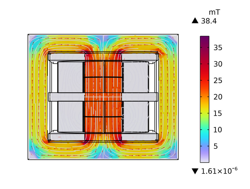
The magnetic flux density concentrated in the core of the transformer for an open-circuit test.

The primary resistance is found to be 76.5 m\Omega as the real part of primary coil impedance. The magnetizing inductance is obtained using the imaginary part of the primary coil impedance and has a value of 44.8 \mu H at 50 kHz.

Short-circuit test

Conventionally, the primary coil is short circuited and the secondary is excited with a voltage reduced enough to pass rated current through the primary coil. In this case, most of the flux is confined to the region of the air gap between the primary and secondary coils. If the secondary coil impedance is computed from the terminal voltage and current values, it mainly consists of the leakage inductance. The leakage inductance can be referred to the primary side using the turns ratio transformation. In the context of the simulation, we can excite the primary and short circuit the secondary coil to directly get the primary leakage inductance.

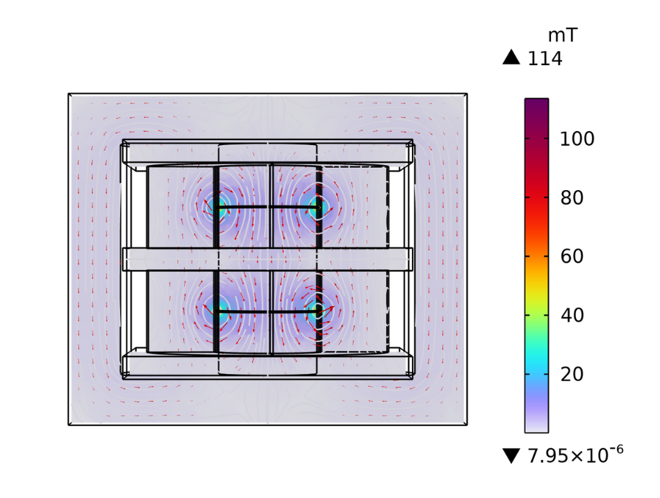
The magnetic flux density concentrated between the primary and secondary coil for a short-circuit test.

The leakage inductance value of 0.25 \mu H is obtained from the imaginary part of the primary coil impedance at 50 kHz. The coil resistance is 19.2 m\Omega.

Computation of Parasitic Capacitances

The transformer is supposed to be a purely inductive device. But, as the primary and secondary coils are made of conducting materials with an insulating layer between them, it can be likened to a case of two conductors separated by a dielectric medium. This gives rise to capacitive effects. As these capacitances are unintended by design, they are referred to as parasitic capacitances. For low-frequency transformers, parasitic capacitances do not play a major role. However, as the frequency increases, capacitive effects become significant; and with a high turns ratio, they start to dominate.

A previous blog post, “How to calculate capacitance matrix”, explains how to get the self-capacitances and mutual capacitances using the Stationary source sweep study step. In the case where the transformers have concentrated windings, this approach can be followed to extract the capacitance matrix.

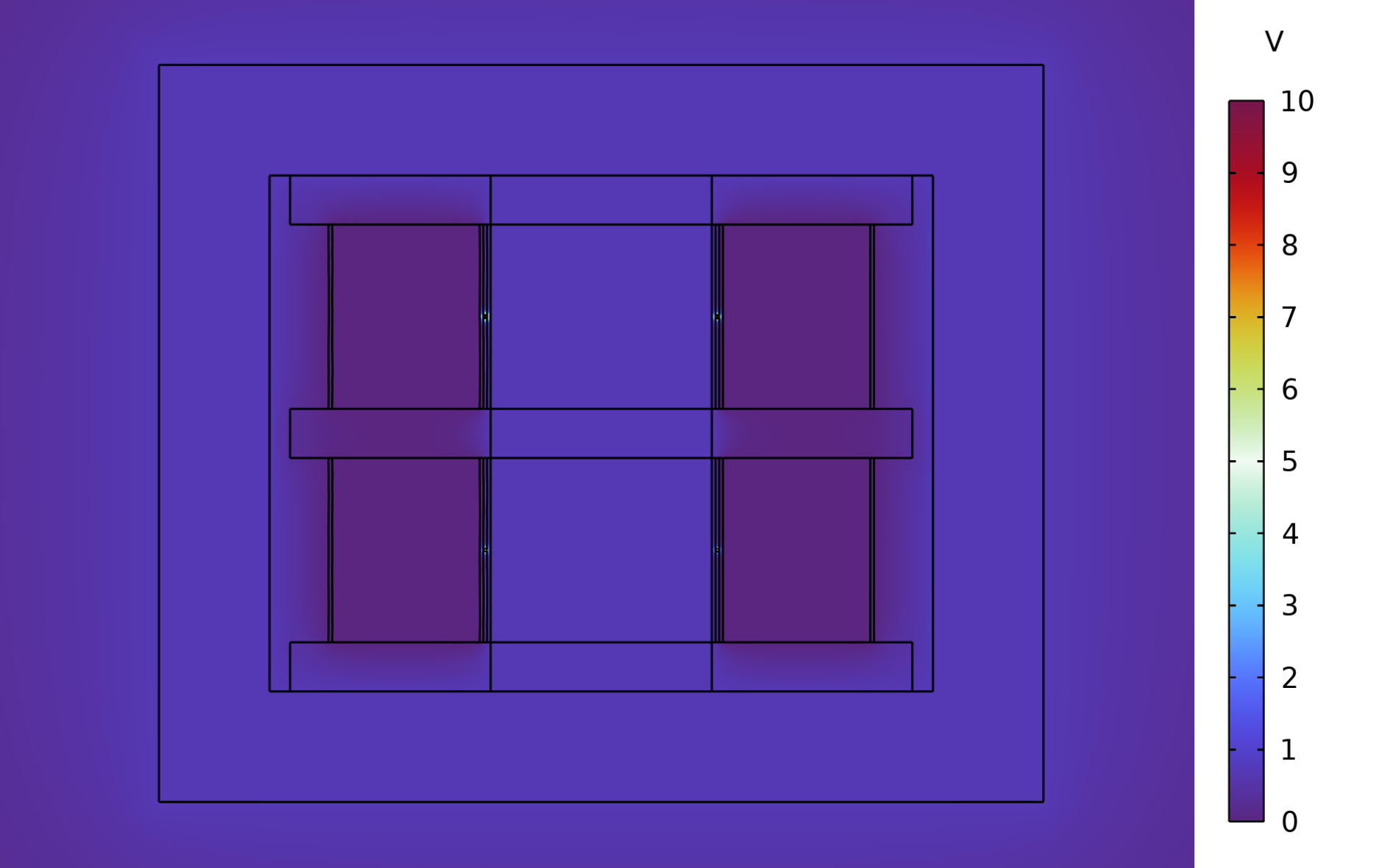
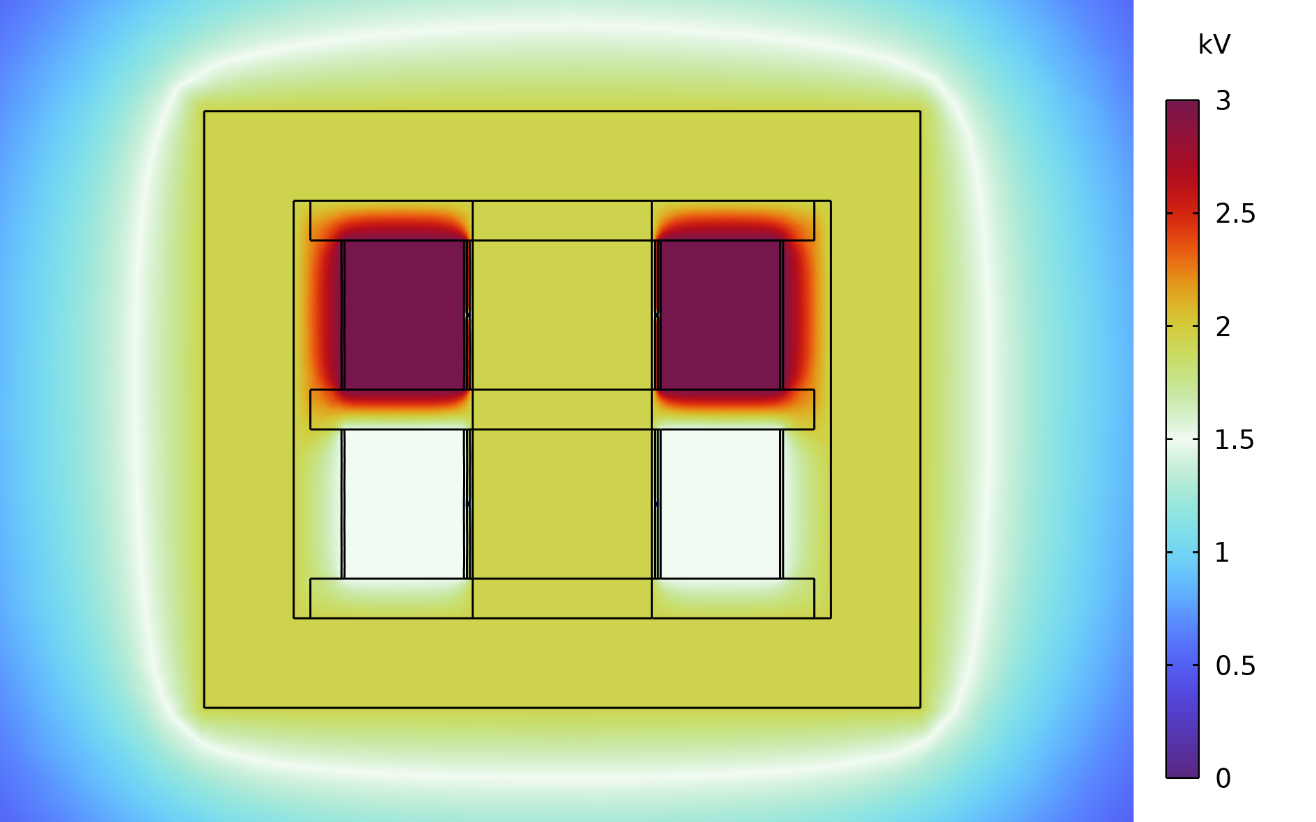
In the present example, the primary and secondary coils are distributed into sections, which is the case for most high-voltage ferrite core transformers. The voltage distribution in the coils exhibits a step change across sections. Hence, the previously described approach is not applicable to extract the capacitance matrix. To compute the primary self-capacitance in this example, we apply half of the potential (i.e., 5 V) to the lower section and full voltage (i.e., 10 V) to the upper section. Ground potential is applied to the secondary coil, and floating potential is applied to the entire surface of the core. The secondary self-capacitance is similarly obtained by applying half of the secondary induced voltage to the lower section and the full voltage to the upper section.

The potential distribution for the primary self-capacitance (left) compared to the potential distribution for the secondary self-capacitance (right).

The computed primary self-capacitance is 14 pF and the secondary self-capacitance is 30.5 pF.

Equivalent Lumped Circuit Analysis

Now that we have the primary resistance, magnetizing and leakage inductance, primary self-capacitance and secondary self-capacitance, we can build an equivalent circuit model of the transformer.

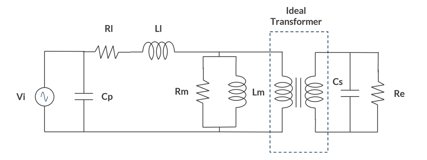
The equivalent lumped circuit of the transformer.

The leakage impedance is represented by a series combination of R_l and L_l. The magnetizing impedance is converted into an equivalent parallel combination of R_m = 2587.6 \Omega and L_m = 44.7 \mu H. The primary and secondary self-capacitances are represented by C_p and C_s, respectively. R_e is an external resistance of 1 M \Omega added to model the open circuit condition of the secondary. Simulation of the lumped circuit model predicts that the primary current has a leading angle of 82.2° and that the secondary induced voltage is 3192 V. It’s important to note that the secondary induced voltage is higher than the value that is expected when using the transformer turns ratio, which is 3000 V. This is observed due to the effect of secondary capacitance combined with the high turns ratio of 1:300. The primary current itself has a leading power factor, implying that the transformer draws a capacitive current!

Coupled Analysis with Inductive and Capacitive Effects

A 2D axisymmetric model of the transformer is created from the 3D model by using the Cross section feature. The 300 individual turns of the secondary are additionally drawn in the geometry for the application of the RLC Coil Group feature, which is available in the Magnetic and Electric Fields interface. The secondary needs to be open-circuited so that the effects of secondary parasitic capacitance can be observed. But if the coil current is specified as zero to make it open-circuited, no current can flow through the secondary self-capacitance. To overcome this, a resistance of 1 M\Omega is connected to the secondary coil using the Electrical Circuit interface. This effectively acts like an open circuit, but allows current to flow through the secondary self-capacitance.

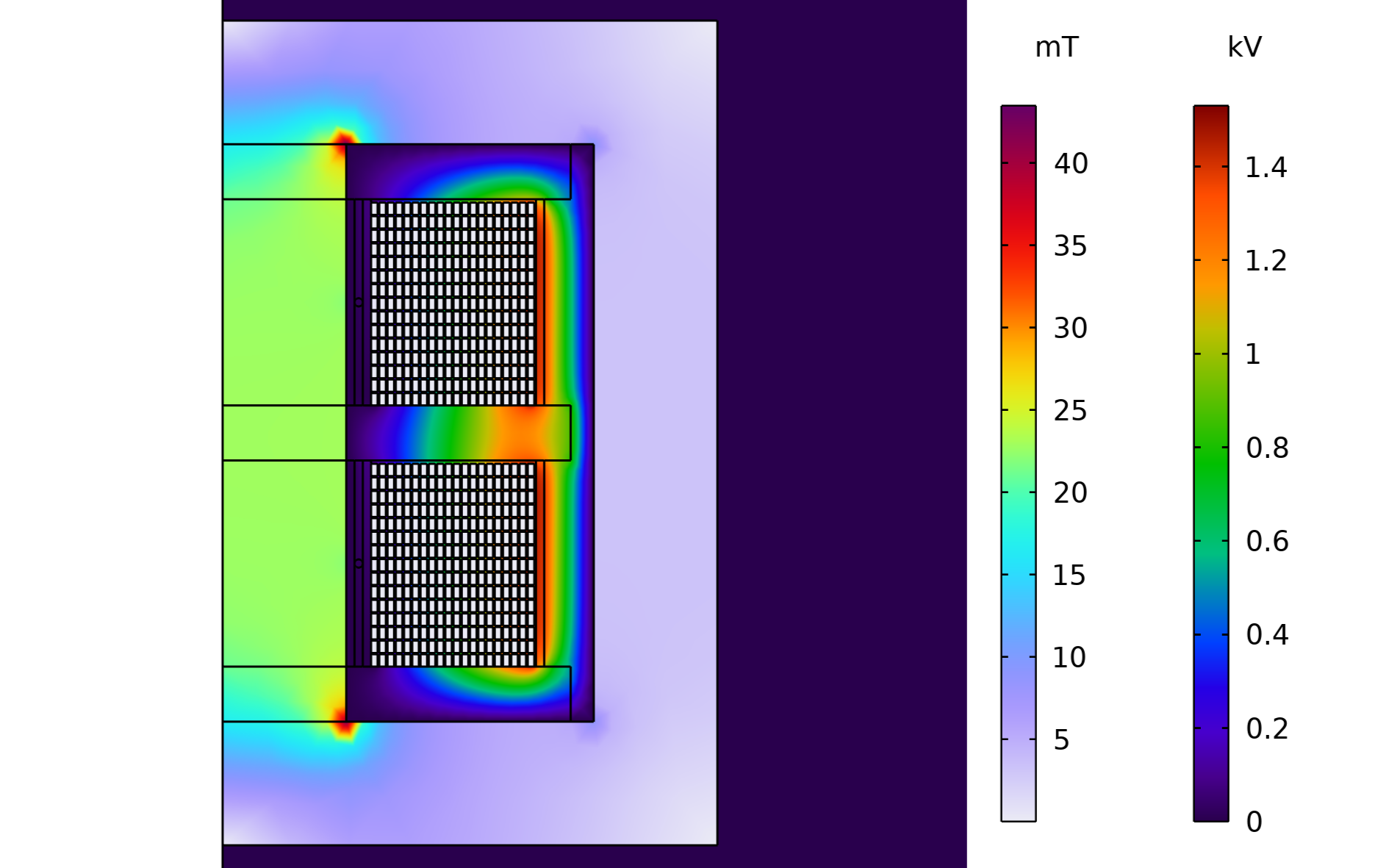
The magnetic flux density and potential distribution.

The potential distribution in the winding region of the transformer shows how the induced voltage goes on increasingly as we move radially outward. From this model, the computed primary current has a leading angle of 75° and secondary induced voltage of 3055.6 V. This is in agreement with the equivalent circuit model discussed in the previous section.

To establish the equivalence of the lumped circuit (derived using the parameters obtained from the 3D model) and the 2D axisymmetric model, the frequency response of the primary coil impedance acquired from the two approaches is plotted on the same graph. The figure below shows how the primary coil impedance magnitude and angle varies with the excitation frequency. We can observe that the 2D axisymmetric results corroborate the ones obtained from the lumped circuit analysis. The lumped electric circuit parameters are extracted from the actual 3D transformer geometry. The 2D axisymmetric model of the transformer is an approximate representation of the actual transformer geometry. These differences result in a slight deviation between the frequency responses of the primary coil impedance obtained from the two approaches.

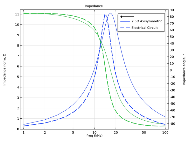
Frequency response of the transformer primary coil obtained from the electric circuit model and the 2D axisymmetric model.

Uses of the RLC Coil Group

This coil modeling feature is used when you want to analyze the effects of in-plane displacement currents. In other words, capacitive effects are to be modeled along with the inductive effects. The connectivity of the turns can be specified using the Domain ordering options. In the case of a transformer, layers of turns pile up radially, and hence column-wise order is chosen.

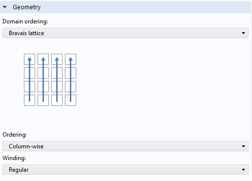
The Domain ordering options for the transformer secondary.

This example uses the built-in options for domain ordering. You can also manually specify it as illustrated in the model: Axisymmetric Approximation of 3D Inductor .

Concluding Remarks

The main objective of the present exercise was to extract the equivalent circuit parameters of a transformer. The magnetizing and leakage inductances were extracted using Magnetic and Electric fields interface. The parasitic primary and secondary capacitances were extracted using the Electrostatics interface.

The RLC Coil Group feature enabled the analysis of a 2D axisymmetric model of the transformer incorporating both inductive and capacitive effects. Simulation of the equivalent lumped circuit as well as the 2D axisymmetric model showed some peculiar results. The computed secondary voltage was more than that expected from the turns ratio. This is similar to the Ferranti effect, found in lightly loaded transmission lines, where the receiving-end voltage rises above the sending-end voltage because of dominant capacitive effects. The primary current of the transformer was also seen to be capacitive in nature. This was due to the domination of secondary parasitic capacitance when referred to the primary by a very high turns ratio of 1:300.

Inductances and capacitances have a mutually opposing effect on the circuit current. An inductive circuit has a lagging power factor whereas a capacitive circuit has a leading power factor. If we attempt to extract the equivalent impedance of such a transformer from the terminal voltage and current, the coupled effects would lead to misleading and erroneous results. As is observed from the 2D axisymmetric model of the transformer, the secondary parasitic capacitance when referred to the primary coil dominates over the inductive effects in the resulting primary coil impedance. At 50 kHz, the transformer effectively behaves like a capacitance.

To conclude, it’s shown here how to extract the equivalent inductances of a transformer separately using analysis of magnetic field effects due to conductive and inductive currents, while ignoring displacement currents. This can be done using the Magnetic fields or Magnetic and Electric fields interface. Similarly, the parasitic capacitances of the transformer can be obtained separately through the analysis of electric fields only. This is possible through either the Electrostatics or Electric Currents interface. It is finally demonstrated how to combine the extracted quantities into a single equivalent lumped circuit model of the transformer.

Next Step

Try the High Voltage Ferrite Core Transformer tutorial model yourself by clicking the button below, which will take you to the Application Gallery entry: