Guidelines for Modeling Rotating Machines in 3D

In a previous blog entry, we showed you how to model rotating machines, like motors and generators, using the Rotating Machinery, Magnetic interface in COMSOL Multiphysics. Today, we will demonstrate the steps we outlined with a 3D generator model example, comparing our results with an analogous 2D model. The concepts of sector symmetry and periodic boundary conditions, including examples illustrating their use, are also highlighted.

Model Example: Permanent Magnet AC Generator

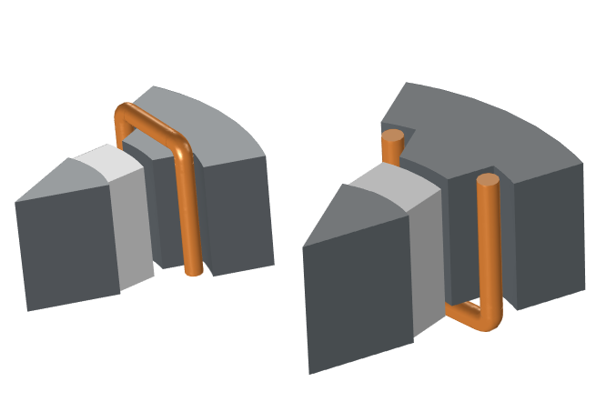
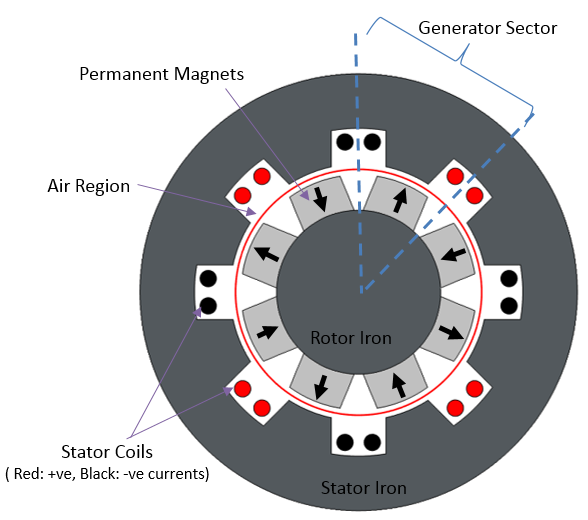
For our purposes, we will focus on a sector of the permanent magnet generator tutorial, available in our Application Gallery. This 2D example can be extended in 3D with a generator stack length of 0.4 m. Since the geometry is symmetric about the rotor axis, we can retrieve results for a full 3D geometry by simply solving a portion of it. This means that only 1/16 of the original geometry must be solved.

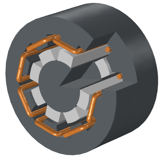
Left: 3D schematic of a generator, with a cutout showing the rotor, stator, and stator windings. Right: A portion of the 3D geometry from two different views.

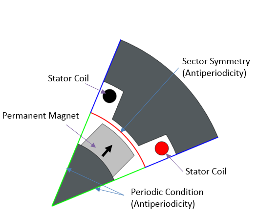
Left: Cross-section geometry of an AC generator in 2D. Right: Sector geometry of the AC generator.

Important Steps for Modeling a 3D Rotating Machine

Using the 3D sector geometry discussed above, we will highlight the key steps behind modeling a rotating machine. For this AC generator example, choose the 3D modeling space and then select the Rotating Machinery, Magnetic interface and the Stationary study type. Next, define your Parameters, including length, number of sectors, wire diameter, and rpm.

Parameters included in the simulation of an AC generator.

Geometry

Rotating magnetic machines consist of two parts: a stator and a rotor. Thus, when modeling such a machine, its geometry must be cut into two parts. This is typically achieved by splitting the air gap between the parts. Two separate unions are formed for the different regions. Form Assembly is used to finalize the geometry, automatically creating identity pairs under Definitions. In 3D, the air region is added around the stator-end winding to capture the fringing fields. (The 2D model does not capture this element.)

Unions of the rotor and stator domains in the geometry sequence.

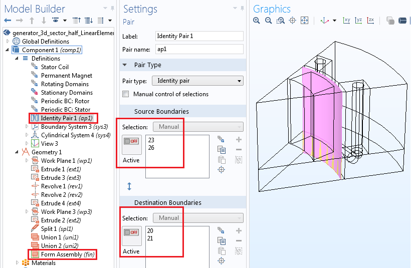
Identity pair settings for separating the stator and rotor domains when the geometry is finalized via Form Assembly. Various selections for domains and boundaries are shown in the Definitions node.

Definitions

In the Definitions branch, define the selections for geometric entities, such as domains or boundaries. Here, we have:

• Stator Coil
• Permanent Magnet
• Rotating Domains
• Stationary Domains
• Periodic BC: Rotor
• Periodic BC: Stator

These selections are reused throughout the model component for physics, meshing, and postprocessing. Within the same branch, you can also define coordinate systems to use in the physics setup.

Rotating Machinery, Magnetic Interface

The Rotating Machinery, Magnetic interface uses two approaches (mixed formulation) to solve Maxwell’s equations: the magnetic vector potential (MVP) and the magnetic scalar potential (MSP). The same formulations are used in the Magnetic Fields and the Magnetic Fields, No Currents interfaces, respectively.

The MSP formulation introduces fewer degrees of freedom and ensures a more accurate coupling of the magnetic flux density when used with a pair feature like Continuity or Sector Symmetry. Therefore, it is important to solve an air region on either side of the identity pair through the MSP. You can do so by utilizing the Magnetic Flux Conservation feature in the Rotating Machinery, Magnetic interface.

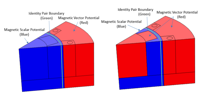
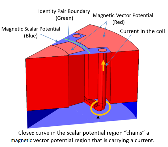
The MSP and MVP regions, along with an identity pair boundary.

In the above image on the left, the stator coil, stator iron, and air region on the stator side are modeled with MVP. The rotor iron, permanent magnet, and air region of the rotor, as well as a part of the stator’s air region, are modeled with MSP. Using this setup, you can model the entire MVP region with the Ampère’s Law feature. Since the MVP formulation allows for current-carrying domains, it is possible to model the stator iron region for the induced eddy currents and compute the eddy current losses. The same, however, cannot be said for the rotor iron, as it is an MSP formulation and explicitly assumes that there is no current in the regions. If you wish to compute the eddy current losses both on the stator and rotor iron (or if you have any other conducting domains in the rotor), you must also solve for those regions with MVP, as illustrated in the above figure on the right.

For both configurations, the MSP regions are simply connected. In other words, they do not include any MSP regions containing a closed loop that “chains” the current-carrying conductor. Illustrated below is an invalid topology example where the entire air region is assigned an MSP. A closed curve in the MSP region “chains” an MVP region that is carrying a current (stator coil). Such a topological issue should be avoided.

Invalid topology where the MSP region is not simply connected.

Let’s start with MSP. To begin, add the first Magnetic Flux Conservation feature and assign it to the rotor side’s air region and the stator side’s air region next to the identity pair. The constitutive relation is set to the linear material with Relative permeability, referencing the Air material in the Materials node.

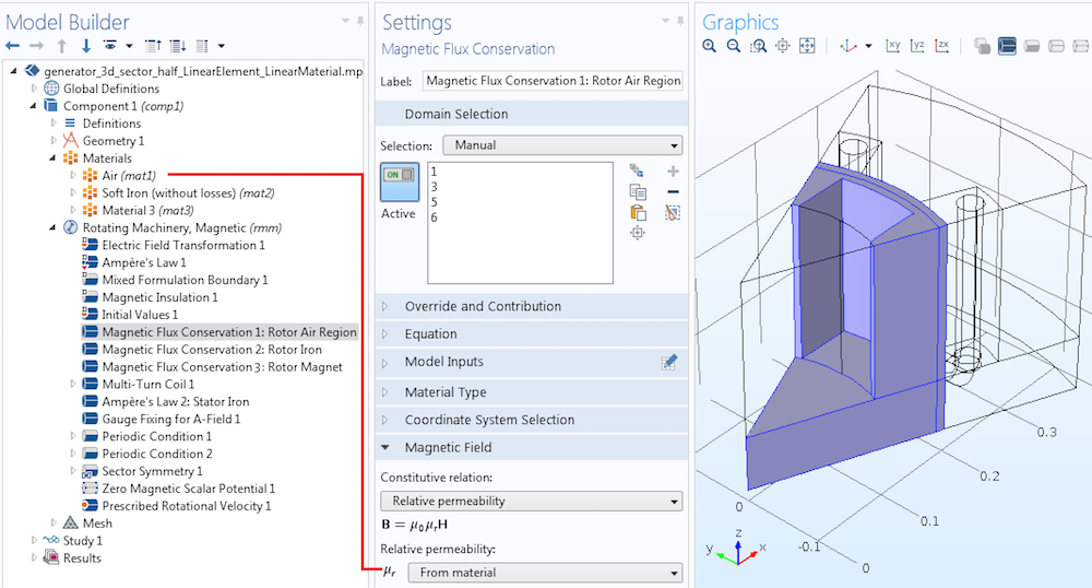
Modeling the air region with MSP.

In the next step, add another Magnetic Flux Conservation feature and assign it to the rotor iron. In the constitutive relation, you can either set it as a linear material with finite (constant) permeability or change it to a nonlinear material using the B-H Curve option. The B-H curve is usually defined in the Materials node, for example, within Soft Iron (without losses). Further, the nonlinear saturation curve can be defined externally with the External Material feature, found in the Materials node under Global Definitions.

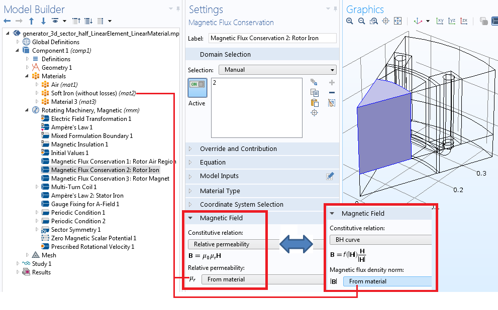
Modeling linear or nonlinear magnetic materials in the rotor.

When it comes to modeling the permanent magnet region, you can do so with the Magnetic Flux Conservation feature. The constitutive relation is set to Remanent flux density or Magnetization. The cylindrical system is used to assign magnetization in the radial direction.

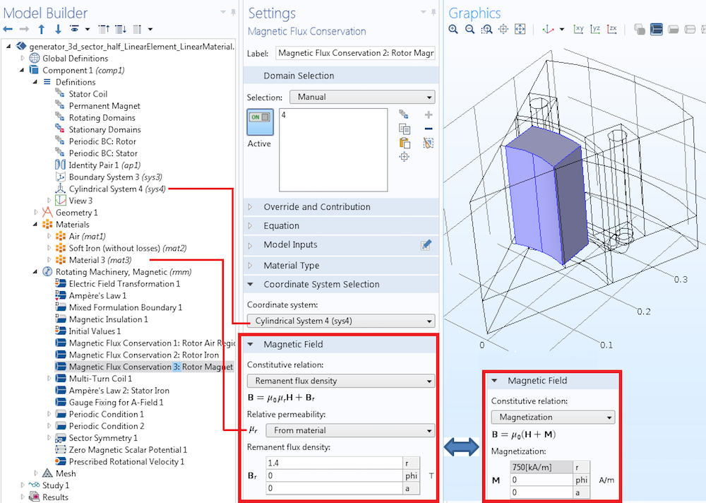
Permanent magnet modeling in the rotor.

To model the stator coil, use the Multi-Turn Coil feature. The coil is set up to measure the open-circuit voltage (the current is zero) in the winding. The total coil length is obtained by specifying the appropriate factor (in our case, 16) for the Coil length multiplication factor, found in the Geometry Analysis subnode within the Multi-Turn Coil feature. The next step involves specifying the Input and Output boundary conditions on the two ends of the stator coil.

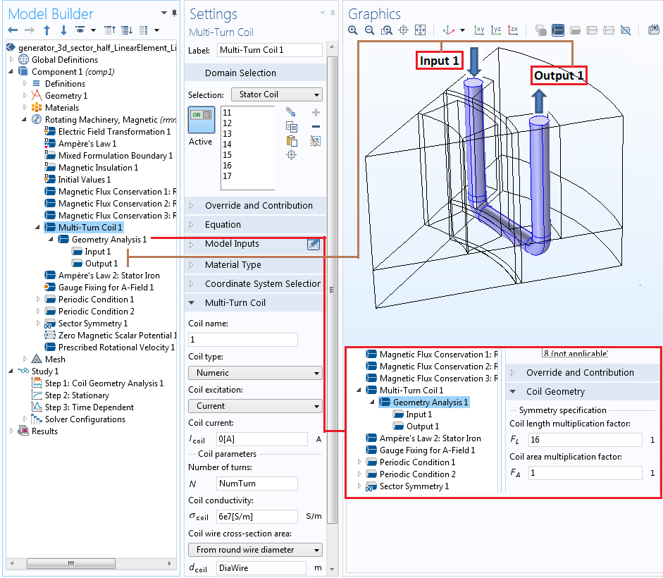
Modeling a stator coil with the Multi-Turn Coil feature. The settings for the Geometry Analysis subfeature and the Input and Output boundary conditions are also shown.

To model the stator iron region, let’s add another Ampère’s Law feature to the model. The constitutive relation can either be set as a linear material with finite permeability using Relative permeability or changed to a nonlinear magnetic saturation curve via the H-B Curve option. Similar to the rotor iron, the H-B curve is typically defined in the Materials node. However, if you have different materials in the stator and rotor, then you need to add two separate nonlinear materials in the Materials node.

Applying Ampère’s Law to the stator iron region. Both the linear and nonlinear material options are highlighted.

For greater numerical stability, you can apply a Gauge Fixing for A-Field feature to every vector potential domain. Say your MVP region is completely enclosed within the MSP region. Or, perhaps, the gauge-fixed domain and its boundaries are interior to the geometry and are not touching the Magnetic Insulation boundary condition. In either of these situations, the gauge fixing needs to be constrained by at least one point. To achieve this, enable the Ensure constraint on value check box in the Advanced Settings section of the feature. The settings are only available if the Advanced Physics Options section is enabled in the Show button, found in the Model Builder. This tutorial offers further insight.

Further, for numerical convergence, you also need to use a nonzero electrical conductivity. This could be, for example, 10 S/m in the Materials node (Air and Soft Iron), where MVPs are used to solve domains.

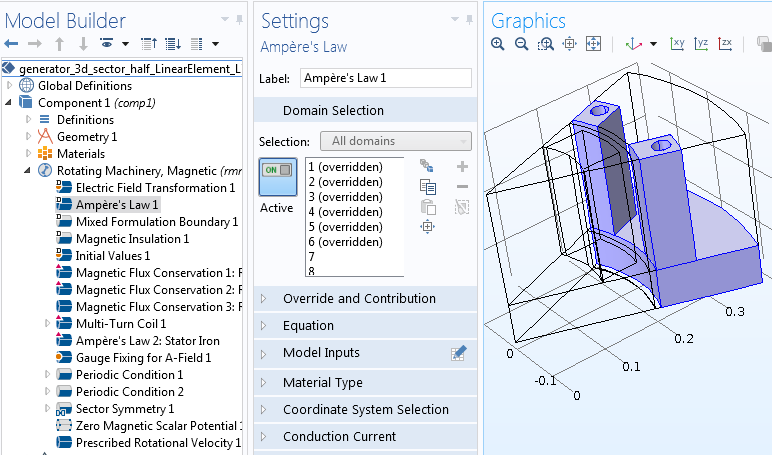
After adding several features to various regions, the default Ampère’s Law is now applicable only for the stator air region that is solved for with MVP. The default Mixed Formulation boundary condition automatically imposes appropriate conditions at the interface between the MSP and MVP regions.

Left: The domain selections for the default Ampère’s Law. Right: The boundary selections for the default Mixed Formulation boundary condition.

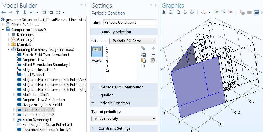
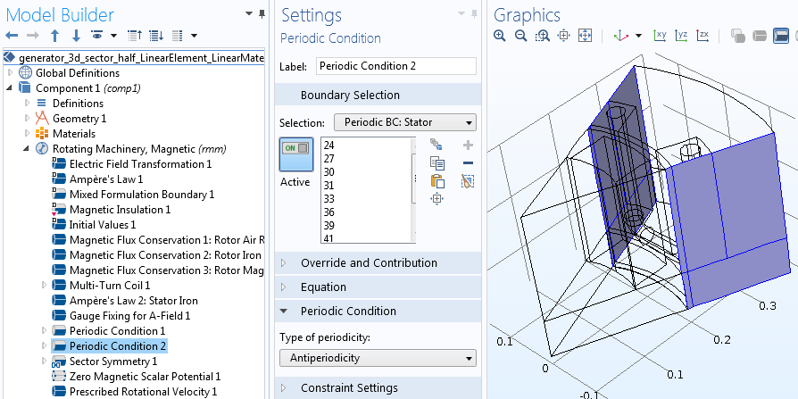
Let’s now apply the periodic conditions on boundaries resulting from cutting the geometry into sectors. If all of the sectors are exactly the same, choose Continuity. If the sectors have the same geometry but their excitations (i.e., permanent magnets or currents) change signs in adjacent sectors, choose Antiperiodicity. The latter is the case for an AC generator example, where adjacent sectors have alternate magnetization. It is recommended that you use two separate periodic condition features, one for the stator and one for the rotor, to ensure that periodic boundaries are properly detected.

Separate periodic conditions are used for the rotor and stator regions.

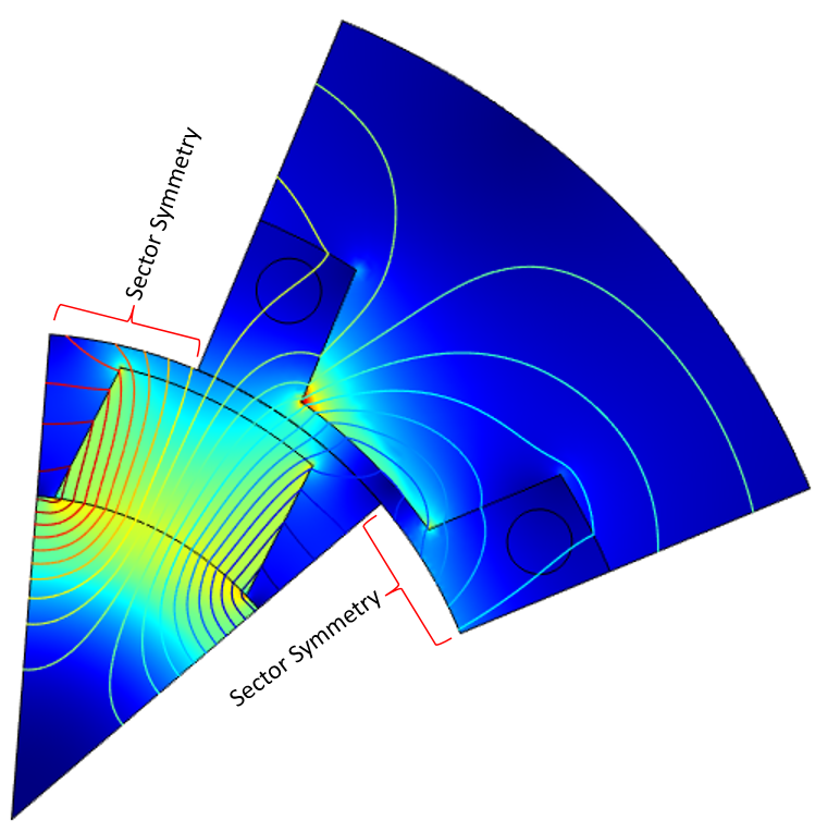
Apply the Sector Symmetry pair condition to the pair connecting the rotor and stator. In the settings window, indicate the number of sectors and the type of periodicity (consistent with the type specified in the periodic conditions). Sector Symmetry works like the Continuity pair feature in regions where the rotor and stator overlap, while applying a cyclic symmetry condition on the nonoverlapping part.

The sector symmetry settings for the Antiperiodicity condition.

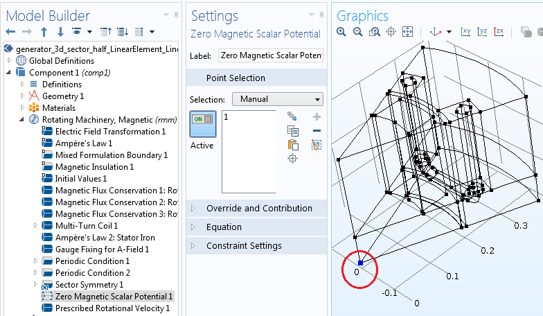
For the solver to converge, you need a unique solution for the MSP. You can achieve this by adding a Zero Magnetic Scalar Potential to one point in the MSP region. If you happen to have two separate MSP regions (i.e., one in the stator and one in the rotor), a one-point constraint must be applied to each region.

Point constraint settings.

Finally, add the rotational motion of the rotor using the Prescribed Rotation or Prescribed Rotational Velocity features. The former is used to specify an angle of rotation, which can be a function of time. The latter is used to enter a constant angular velocity, with the angle increasing linearly as a function of time.

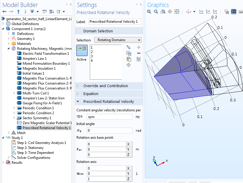
Prescribed rotation of the rotor domains around the z-axis.

Meshing

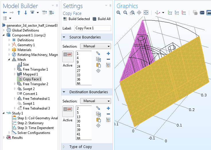
Whenever you have a periodic condition in your model, the mesh must be identical on the source and destination boundaries. Initially, a Free Triangular or Mapped mesh should be applied to the source boundaries. Then, using the Copy Face feature, you can copy the same mesh onto the destination boundaries.

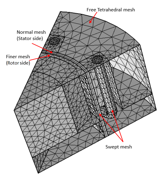
Additionally, to accurately map field quantities from source to destination boundaries in the identity pair, there needs to be a finer mesh on the destination side (rotating boundary) than on the source side (stationary boundary). To get full control, it is helpful to mesh the surfaces separately.

By using a Swept or Mapped mesh whenever possible, you can significantly reduce the number of mesh elements. A free triangular mesh is first applied to one end of the Multi-Turn Coil feature, and a swept mesh is applied to the entire coil region. Similarly, a swept mesh is also used for part of the air region between the stator and rotor.

Left: Copy Face feature settings for source and destination boundaries at the periodic conditions. Right: Final mesh used in the 3D generator sector model.

Solver Settings

The Rotating Machinery, Magnetic interface supports two types of study steps: Stationary and Time Dependent. For time-dependent simulations, it is critical to have an accurate initial value that corresponds to the physical situation. For example, if you have a permanent magnet in your model, you must first solve a stationary step, using the solution as the initial values for the time-dependent study.

For the 3D AC generator sector, we set up our study in three different steps:

1. Coil Geometry Analysis: Computes the coil current direction for the numeric coil type used in the Multi-Turn Coil feature
2. Stationary: Computes the static magnetic fields generated by the rotor’s permanent magnets
3. Time Dependent: Performs a transient simulation of a generator, with the solution from the previous step used as the initial values

Improve Simulation Performance

You can improve the simulation’s performance by choosing different discretization orders of the finite element mesh applied to the model. The default discretization order is quadratic for both MVP and MSP. Setting the discretization order to linear can, however, significantly reduce the computational time.

To modify the discretization order, you first need to enable Discretization by clicking the Show button. The discretization order can then be changed to linear via the Rotating Machinery, Magnetic interface for one or both of the dependent variables: MVP and MSP.

Results

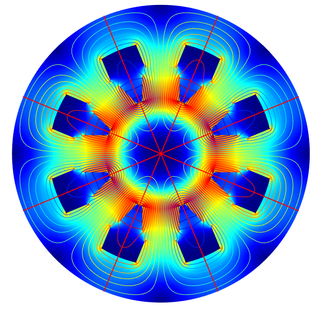
After solving, you can look over the geometry using the Sector 2D and Sector 3D data sets. To add the sector data sets, right-click on Data Sets under the Results node. Specify the number of sectors and if the model is antiperiodic. Next, select the Invert phase when rotating check box in the Advanced section. Any plots using this data set will show the reconstructed geometry in its entirety. If you have a model with mirror symmetry, like the example discussed here, you can use the Mirror 3D data set to obtain the solution for the other half of the full model. Note that the Mirror 3D data set can be added either before or after the Sector 3D data set.

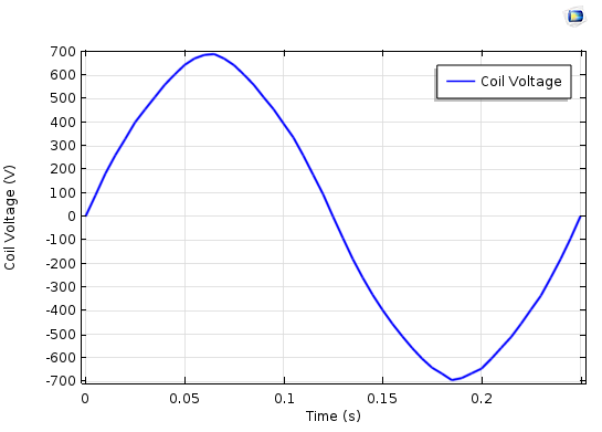
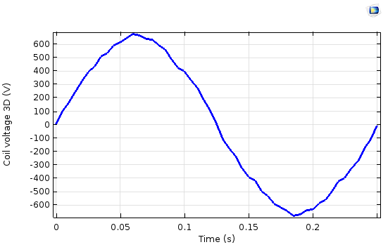
It is possible to directly evaluate the induced voltage in the stator coil using the variable rmm.VCoil_1, found in the Global plot under 1D Plot Group. To get the total induced voltage in the stator coil for a 2D sector model, you have to multiply the variable by the number of sectors (eight). This is taken care of in the 3D sector model via the Coil length multiplication factor.

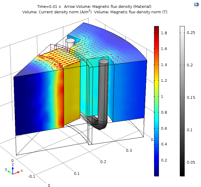
Left: Magnetic flux density (T) and field lines in the sector model during rotation. Right: Complete geometry reconstructed using a Sector 2D data set. The red lines indicate the separation between the different copies of the sector geometry.

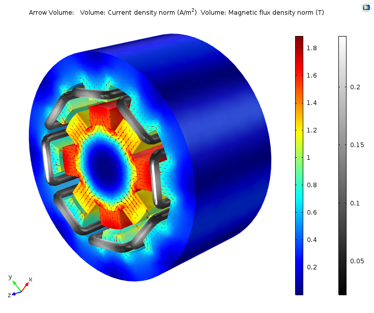
Left: Magnetic flux density (volume and arrow volume) in the permanent magnet and irons, along with the current density (gray scale) in the sector model’s stator coil at t = 0.01 s. Right: Complete geometry reconstructed using the Mirror 3D and Sector 3D data sets.

Left: The induced stator coil voltage in the 2D sector model using the nonlinear magnetic material and quadratic mesh elements. Right: The induced stator coil voltage in the 3D sector model using the nonlinear magnetic material and linear mesh elements.

Next Steps

• Download the tutorial models presented here and try them out:
• Generator sector in 2D and 3D
• Generator in 2D
• Check out the other blog posts in our Electromagnetic Device series
• Interested in modeling rotating machines in COMSOL Multiphysics? Contact us today