
In fluid flow simulations, it is often important to evaluate the forces that the fluid exerts onto the body — for example, lift and drag forces on an airfoil or a car. Engineers can use these body forces to quantify the efficiency and aerodynamic performance of designs. Today, we will discuss different ways to compute lift and drag in COMSOL Multiphysics.
Defining Lift and Drag
When fluid flow passes a body, it will exert a force on the surface. As shown in the figure below, the force component that is perpendicular to the flow direction is called lift. The force component that is parallel to the flow direction is called drag. For simplicity, let’s assume that the flow direction is aligned with the coordinate system of the model. Later on, we will show you how to compute the lift and drag forces in a direction that is not aligned with the model coordinate system.
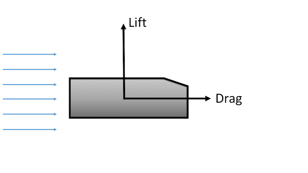
Schematic of lift and drag components when fluid flow passes a body.
There are two distinct contributors to lift and drag forces — pressure force and viscous force. The pressure force, often referred to as pressure-gradient force, is the force due to the pressure difference across the surface. The viscous force is the force due to friction that acts in the opposite direction of the flow. The magnitudes of pressure force and viscous force can vary significantly, depending on the type of flow. The flow around a moving car, for instance, is often dominated by the pressure force.
Computing Lift and Drag Using Total Stress
COMSOL Multiphysics offers complete access to all of the internal variables and makes it very easy to compute surface forces via integration on a boundary. Here, we will demonstrate how to compute the drag forces on an Ahmed body. You can download this model from our Application Gallery.
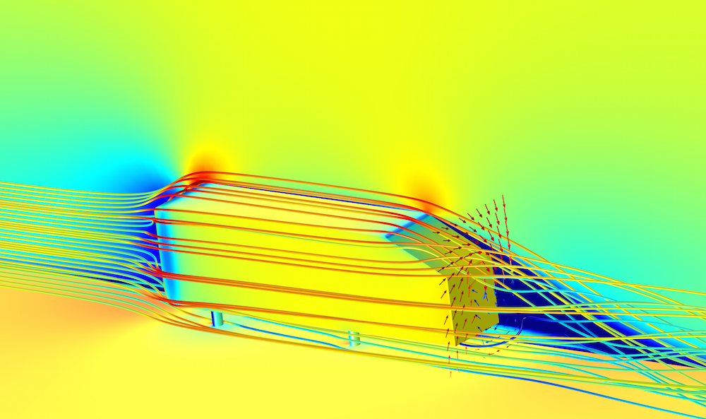
Simulation of airflow over an Ahmed body. The surface plot shows the pressure distribution, and the streamlines are colored by the velocity magnitude. The arrow surface behind the Ahmed body shows the circulation in the wake zone.
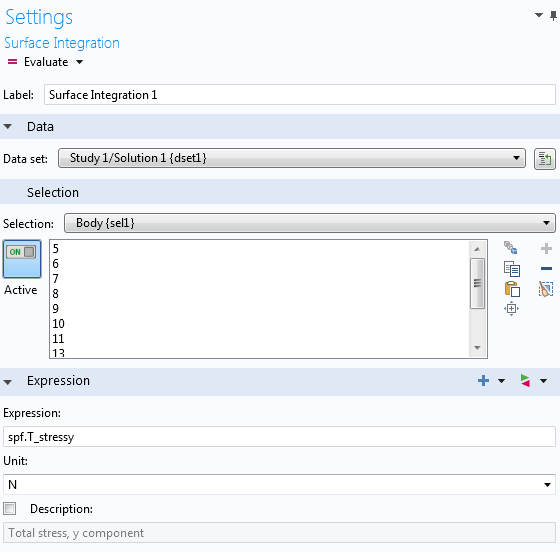
There are several ways to compute drag depending on the physics. The most straightforward way is to integrate the total stress — which includes contributions from the pressure force and the viscous force — in each direction. To do so, we first need to define a surface integration operator under the Derived Values node, as illustrated below.

TIP: Alternatively, you can also use a boundary probe or integration operator in the component coupling to define such integration. The difference is that the operations defined in the physics setting can be used during the simulation — for example, drag force computed with a boundary probe as an objective or a constraint in an optimization study.
Next, we can select the boundaries to perform the integration. In this example, we chose all of the boundaries on the body. Drag in this model is in the y-direction. We can type in the expression: spf.T_stressy, which represents the total stress in the y-direction.
Computing Pressure Force and Viscous Force Separately
Sometimes, engineers can obtain greater insight into designs by examining the pressure force and viscous force separately. COMSOL Multiphysics features a predefined variable, spf.K_stressy, for viscous stress in the y-direction. We can readily evaluate the viscous force by integrating the viscous stress.
What about the pressure force? Pressure, denoted by the variable p, is a scalar. To project in the direction of drag, we need to multiply pressure by the y-component of the normal vector on the surface, spf.nymesh. Therefore, we can evaluate the pressure force by integrating spf.nymesh*p on the surface.
In some special turbulent flow cases where the wall function is used, it is more accurate to compute the viscous force using the friction velocity, spf.u_tau. In COMSOL Multiphysics, the k-epsilon and k-omega turbulence models use the wall function.
To learn more about turbulence models in COMSOL Multiphysics, read our blog post “Which Turbulence Model Should I Choose for My CFD Application?“.
We can obtain the local shear stress at the wall by:
Therefore, the local shear stress in the y-direction is:
where u^T is the tangential velocity at the wall. We can further rewrite u^T as u_\tau*u^+, where u^+ is the tangential dimensionless velocity.
Without going into too many details on derivation, we can translate the previous equations into COMSOL variables. We can integrate the local wall shear stress in the direction of drag (the y-direction) with the following expression: spf.rho*spf.u_tau*spf.u_tangy/spf.uPlus. In this expression, spf.rho is the density of the fluid, spf.u_tangy is the velocity in the y-direction at the wall, and spf.uPlus is the tangential dimensionless velocity.
The table below summarizes the expressions used to compute each force.
| Fluid Flow Without Wall Function | Turbulent Flow with Wall Function | |
|---|---|---|
| Pressure Force | spf.nymesh*p | spf.nymesh*p |
| Viscous Force | -spf.K_stressy | spf.rho*spf.u_tau*spf.u_tangy/spf.uPlus |
| Total Force | -spf.T_stressy | spf.nymesh*p + spf.rho*spf.u_tau*spf.u_tangy/spf.uPlus |
Note: In this example, the drag force is in the y-direction. You may need to change the projection direction based on the orientation of your model.
Correction for Angle of Attack
It is common that the geometry may not be aligned perfectly with the flow direction. The angle between the center reference line of the geometry and the incoming flow is called angle of attack (often denoted by the Greek letter \alpha). In aerospace engineering, the angle of attack is frequently used as it is the angle between the chord line of the airfoil and the free-stream direction. The following figure shows the relationship between lift, drag, and angle of attack on an airfoil.
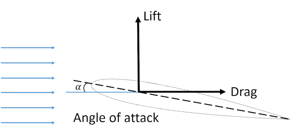
Schematic illustrating lift, drag, and angle of attack on an airfoil.
Using a 2D NACA 0012 model, we will show you how to compute lift with an angle of attack correction. This model is available for download in our Application Gallery.
There are two ways to change the angle of attack of the model. We can either rotate the geometry itself or we can keep the geometry fixed but modify the flow direction at the inlet. Here, we will use the second approach. It is much simpler to adjust the velocity field at the inlet boundary condition as we would not need to remesh the model for each angle of attack. As shown in the figure below, the airfoil is fixed while the streamlines show the flow at an angle of attack due to the adjusted inlet velocity direction.
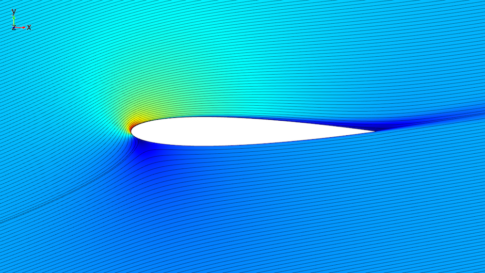
Simulation of flow passing a NACA 0012 airfoil at a 14-degree angle of attack. The surface plot shows the velocity magnitude along with the streamlines (shown in black).
This example uses the SST turbulence model, which does not use the wall function. Therefore, we will use total stress to compute lift. At a zero angle of attack, the lift is simply -spf.T_stressy. If the angle of attack is nonzero, we can project the force onto the direction of the lift using the following expression: spf.T_stressx*sin(alpha*pi/180)-spf.T_stressy*cos(alpha*pi/180). Here, alpha represents the angle of attack in degrees.
What About Lift or Drag Coefficients?
You may also be interested in the nondimensionalized forms of lift and drag — the lift coefficient and the drag coefficient. It is often easier to use the coefficients instead of the dimensional forces for the purpose of validating experimental data or comparing different designs. The lift coefficient in 2D is defined as:
Since we have already calculated the dimensional lift, we can simply normalize the lift by the dynamic pressure and the chord length. With the dimensionless lift coefficient, we can compare our simulation results with experimental data (Ref. 1).
Note: In 3D, the lift coefficient is nondimensionalized by area instead of length: C_L = \frac{L}{\frac{1}{2} \rho u^2_\infty A}
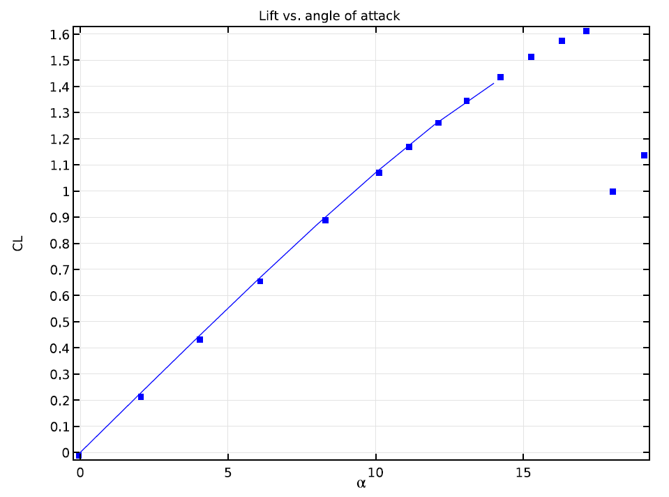
Graph comparing simulation results and experimental data of the lift coefficient on a NACA 0012 airfoil at various angles of attack.
As illustrated in the above graph, no discernible discrepancy between the computational and experimental results occurs within the range of the angle of attack values used in this simulation. The experimental results continue toward a high angle of attack regime where the airfoil stalls.
Concluding Remarks
In this blog post, we have explored ways to compute lift and drag on an Ahmed body and an NACA 0012 airfoil. We have demonstrated how to compute pressure force and viscous force, while also examining the special case where a wall function is used in the turbulence model.
Each of the approaches we have presented here are certainly not limited to these specific simulations. You can compute the body forces on any boundaries or surfaces, thereby gaining insight into designs through multiphysics simulations. With the Optimization Module, you can take this analysis one step further and optimize lift or drag.
References
- C.L. Ladson, “Effects of Independent Variation of Mach and Reynolds Numbers on the Low-Speed Aerodynamic Characteristics of the NACA 0012 Airfoil Section,” NASA TM 4074, 1988.


Comments (19)
Abimbola Ashaju
June 23, 2015when integrating your total stress, what factor do you consider in choosing either of volume, surface or line integral
Peter Lyu
June 23, 2015 COMSOL EmployeeHi Abimbola,
You would use line integration for 2D simulations and surface integration for 3D.
Peter
Sathish Sanjeevi
October 25, 2016Hi,
Could you also update, how to compute Torque acting on the particle?
Best Regards,
Sathish
Peter Lyu
November 9, 2016 COMSOL EmployeeHi Sathish,
Thank you for your comments. Computing torque on particles is quite specific and depends on the physics interface used. Please contact us at support@comsol.com and we can assist you further.
Peter
Sathish Sanjeevi
January 19, 2021Hi Peter,
Through some online reading, I am able to compute Torque acting on a particle. I am posting it here for interested users. For example, to compute Torque acting about x-axis, it can be computed using cross product and is given by -(spf.T_stressz*y-spf.T_stressy*z).
Sathish
Vishal Anand
July 16, 2021Thanks Satish.
However I have a doubt. The actual torque should be about the center of mass of the particle and therefore the moment arm of the torque should only be measured about COM. In that case, how do we find out the COM of the particle to find the torque?
mohamed fahmi arfaoui mohamed fahmi arfaoui
January 26, 2017Comment fait une simulation du profil aérodynamique NACA 0012 avec angle d’attaque variable pour comsol 4.2
Bridget Cunningham
February 9, 2017 COMSOL EmployeeHello,
Thank you for your comment.
For questions related to your modeling, please contact your local support team.
Online support center: https://www.comsol.com/support
Email: support@comsol.com
Best,
Bridget
Ignaas Jimidar
June 20, 2017Hello Peter,
Thanks for this nice description. However, I have one remaining question: are you calculating the viscous force and total force of the fluid on the body or the other way around? Because in the summary table, you put a minus sign, and this confuses me a bit…
Best,
Ignaas
Asutosh
September 12, 2017Dear Peter Lyu,
Thanks for providing the valuable information. However It’s quite confusing about the -ve sign in lift and drag expressions. I was simulating incompressible laminar flow around a 3d model along Y-direction with “no slip boundary” condition and calculating lift and drag with “spf.T_stressz”, “spf.T_stressy”. The derived results were in -ve value.
Please let me know if I am following the correct procedures and expressions.
Thanks
Caty Fairclough
January 25, 2018Hi Asutosh,
Thanks for your comment.
The sign dependents on if you are evaluating the force on the structure or on the fluid. You can choose the sign depending on what you want to evaluate. For the lift force, it is the force on the solid that you want to compute so you should use -spf.T_stressy.
Navai Mehdiyev
January 18, 2018Hi Peter,
I’m trying to simulate CFD effects of inclination angle on transport&reaction in hollow cylinder catalyts but when I incline the catalyst particle even by 1 degree it does not work. Could you be so nice as to give me a hint if sth else should be changed in geometry or there’s other way around? Since the study isn’t only about drag coefficient, changing flow direction isn’t enough.
Regards,
Navai
Caty Fairclough
January 25, 2018Hi Navai,
Thanks for your interest in this blog post.
For questions related to your modeling, please contact our Support team.
Online support center: https://www.comsol.com/support
Email: support@comsol.com
Sergio Carrasco
September 3, 2018Hello,
How could I compute the drag coefficient over the ahmed surface?
Thank you for your asistance.
Mathias Fortuna
January 17, 2020Hi Peter, how can I find the center of pressure in this kind of studies?
Thanks in advance!
Ahmad Abosrea
December 26, 2020Hi Peter,
For 2D models, is it possible to calculate a compined Drag Coefficient from both x and y directions?
Rajesh Kumar
July 22, 2021How to calculate viscous drag in x-direction? Is it possible to get viscous stresses in the x-direction (using wall function) after replacing y by x and u by v in tau terms I am getting error while using inbuilt stress in comsol.
ARVIND BAIRWA
October 1, 2021Hello Peter Lyu,
I am calculating the drag coefficient of an array of cylinders (120 cylinders).
I am using this expression,
sum( -reacf(u)*2, x, 1,120)/(spf.rho*U_mean^2*d)
which says drag force summation from 1 to 120 cylinder having ‘U_mean’ velocity and ‘d’ diameter. However, it does not seem to work. Could you please suggest a correction in this expression?
Thank you
Steve Kooiman
November 2, 2021Hi Peter,
Thank you for the clear explanation, it is very useful.
In your blog you mention to use “spf.nymesh” to get y-normal component. In the blog “How to Calculate Mass Conservation and Energy Balance” they use “spf.ny” in stead of “spf.nymesh”. What is the difference between them? When do you use ny and when nymesh?
With kind regards,
Steve