
If you have ever imported a mesh into the COMSOL Multiphysics® software, you might have found yourself wondering if there is any way to modify the mesh without going back to the source of the mesh. The Refine and Adapt operations are two useful tools for doing just that. These operations are also available for imported meshes. In this blog post, we demonstrate how these operations work and how you can use them to get the most out of your imported meshes. In the blog post “Editing and Repairing Imported Meshes in COMSOL Multiphysics®”, you can find further examples of how the operations can be used.
Editor’s note: This blog post was updated on September 8, 2022, to reflect new features and functionality in COMSOL Multiphysics version 6.0. The new text was provided by Hanna Gothäll, a senior product specialist for geometry and meshing on our development team.
The Refine Operation
The Refine operation provides a convenient and quick way of reducing the element size in an imported mesh. As the name suggests, the operation essentially partitions the elements that are already present in the mesh. In the Settings window, as shown below, we can select the number of refinements to perform and a bounding box for the operation. It is also possible to perform the operation on the entire mesh or a selection of domains, boundaries, or edges. However, the option that we will discuss in this blog post is Refinement method, for which there are two settings to choose from:
- Split longest side
- Regular refinement
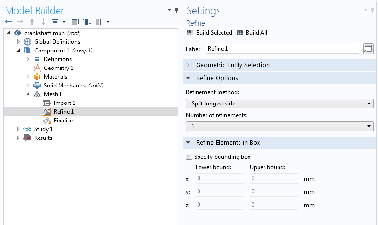
The Settings window for the Refine operation. It’s possible to specify Geometric entity level, Refinement method, Number of refinements, Face representation, and a bounding box for the operation.
To demonstrate how these methods work and what the differences are, let’s have a look at the case of a single tetrahedral mesh element. In the figure below, the plot in the middle shows the element after one refinement step using the Split longest side method. The operation partitions the longest mesh edge of the element into two equal pieces. The element is then divided in two using the new mesh edges. Note, however, that when you have several connected elements, this will lead to some elements being split into more than two new ones to preserve a conforming mesh (not shown in the figure below).
The plot on the lower-right shows the same tetrahedral element partitioned using the Regular refinement method. This time, every mesh edge has been divided into two and then used to split the element into several smaller elements of the same type. For a tetrahedron, this results in eight new elements where there was previously only one. The Regular refinement option also has the capability to preserve the structure in structured meshes, so if you’re importing a structured mesh, this might be something to take into consideration.
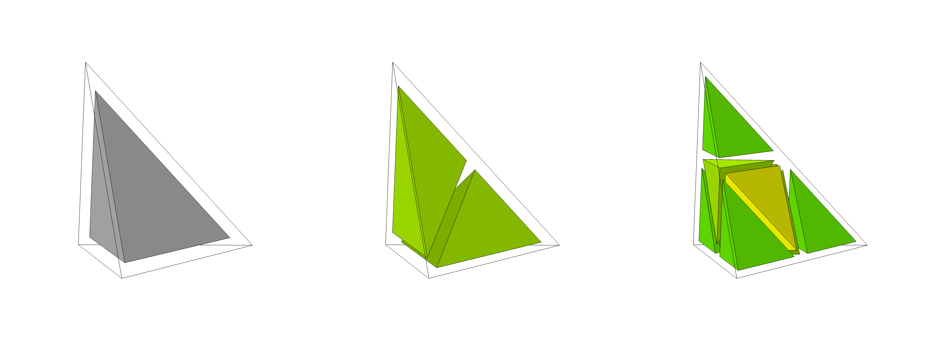
Three mesh plots of a single tetrahedral mesh element before and after building the Refine operation. Left: Unpartitioned element. Center: Element partitioned using the Split longest side setting. Right: Element partitioned using the Regular refinement setting. The element colors in the center and right figures indicate mesh element quality.
The Adapt Operation
Now, let’s have a look at the Adapt operation. While it includes a lot of functionality and can be used for different purposes, we will focus on how you can use the Absolute size expression to modify the element size of your imported meshes.
For more information on using the Adapt operation in conjunction with error estimates and solution data, check out a previous blog post on using adaptive meshing for local solution improvement and the tutorials listed at the end of the article. Additionally, the blog post “2 Mesh Adaptation Methods: Enabling More Efficient Computations” shows how to use Adapt when dealing with anisotropic elements.
We’ll start by looking at how you can apply the Adapt operation to work with the sizes of your elements. The mesh we will be using has been saved to the NASTRAN® file format and can be found in the Eigenvalue Analysis of a Crankshaft tutorial model. Like with the Refine operation, Adapt requires all mesh elements to be linear, so, to start, we’ll make sure to select Import as linear elements in the Import operation. We then add an Adapt feature node, where we select Absolute size for Type of expression.
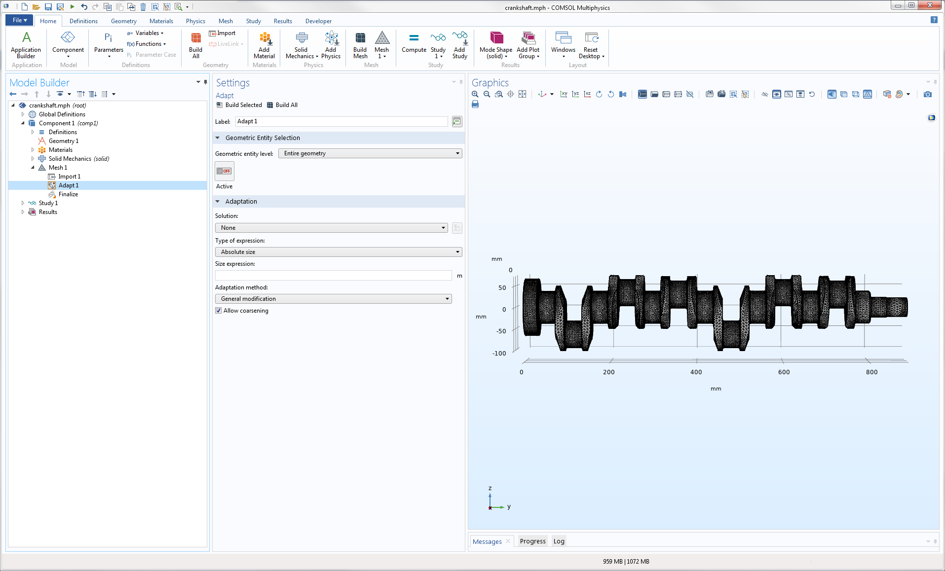
The crankshaft mesh is imported from the NASTRAN® format using the option Import as linear elements. An Adapt node has been added to the sequence of Mesh operations. Here, you can see the Settings window for this node, with the Solution and Type of expression sections set to None and Absolute size, respectively.
Whereas the Refine operation simply partitions all elements to create a finer mesh, by selecting Absolute size, the Adapt operation will try to modify the mesh to make the size of the elements conform to the expression we provide. To achieve this, there are three different methods that can be selected from the Adaptation method menu:
- Longest edge refinement
- Regular refinement
- General modification
Longest Edge Refinement and Regular Refinement
The functions of Longest edge refinement and Regular refinement are based on essentially the same principles as the Refine operation. However, while Refine partitions all elements in the mesh, the Adapt operation will make the mesh conform to the size expression. Thus, if you have elements in your mesh that already closely match the expression or are smaller, they will generally be kept unaltered.
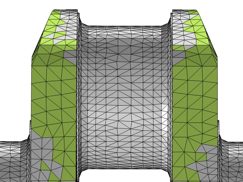
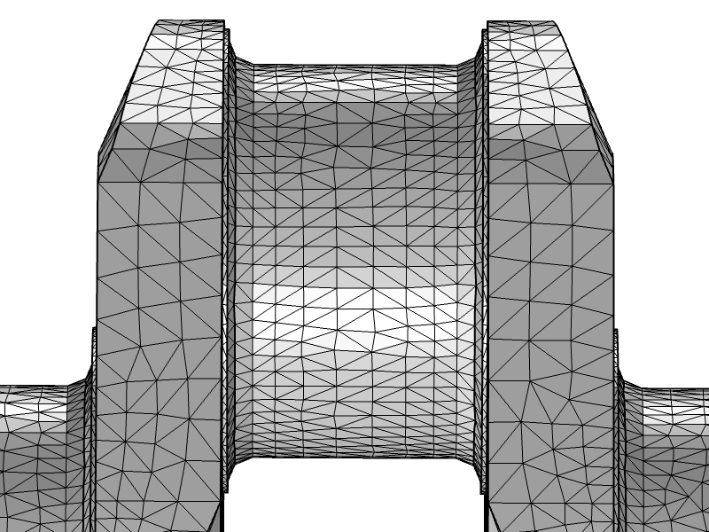
In this way, the Adapt operation prevents unnecessary memory usage by not refining the parts of the mesh where the resolution is already satisfactory. For example, say we want to make the larger elements of the crankshaft mesh finer. One option is to use the Refine operation and set it to Split longest edge and Number of refinements and set it to 1, which will increase the number of elements in the mesh by a factor of about 3.5. Alternatively, we can use Adapt with Longest edge refinement and a Size expression of 8 [mm] to achieve the same size reduction in the desired elements with an increase of less than a factor of 2 in the total number of elements.
A section of the crankshaft mesh before (left) and after (right) running Adapt with the Longest edge refinement setting and the Size expression 8 [mm]. Note that not all elements have been partitioned; only those larger than the size specified in the expression (colored in green in both images) have been.
General Modification
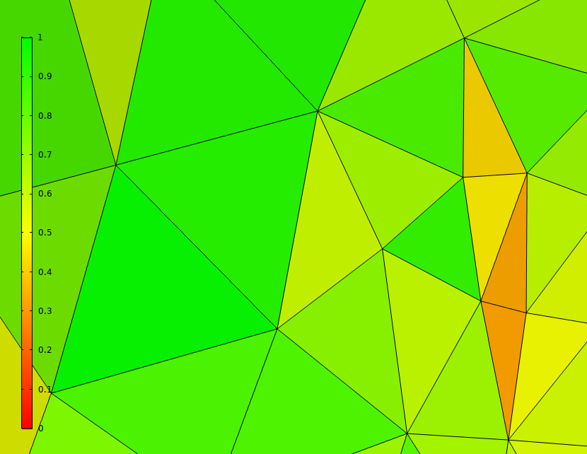
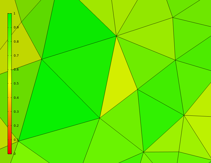
Using the General modification setting, in addition to creating new elements by partitioning elements, the operation is able to move mesh vertices and collapse elements that are too small to coarsen the mesh. As such, while attempting to make the mesh fit the size expression, it tends to make the elements more isotropic, thereby eliminating some poor-quality elements. This makes for a very versatile and powerful tool, as we shall see in this blog post.
A section of mesh before (left) and after (right) applying Adapt with the General refinement setting. The color indicates element quality, which can be seen to clearly increase as small elements are collapsed and vertices are moved.
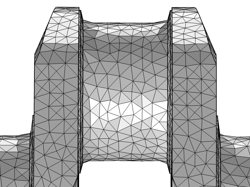
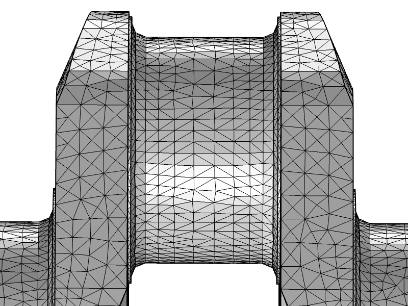
In the example below, you will see the benefits of using General modification. We begin with an unmodified crankshaft mesh on the left. The middle figure shows what the mesh looks like after building Adapt using General modification and a Size expression of 8 [mm]. For the purpose of comparison, the figure on the right shows the results of using Longest edge refinement with the same expression. Notice that for General modification, the operation has moved the mesh vertices. This results in more isotropic and higher-quality elements.
Left: A section of the unmodified crankshaft mesh. Middle and right: The Adapt operation has been applied with the Size expression 8 [mm], using General modification and Longest edge refinement, respectively. Notice how General modification has coarsened parts of the mesh and moved vertices to better fit the expression and improve quality.
Additionally, say that you would like to run a quick simulation to get an estimate of the results. Then, General modification can, with an appropriate Size expression, be used to coarsen the mesh, reducing the number of elements and thereby the computation time.
Modifying the Boundary Mesh
When using the Refine or Adapt operation on an imported 2D or 3D mesh, the operation will create a spline curve for each geometric edge of the input mesh. The operation will use these splines to determine the positions of the edge mesh vertices of the refined or adapted mesh. The figures below indicate that the new mesh vertices that appear on the boundary reside on a spline rather than just residing on the input boundary mesh.
Using a spline curve that is based on the mesh vertices of the input mesh boundary (left) determines the positions of the new mesh vertices on the refined mesh boundary (right).
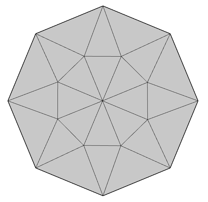
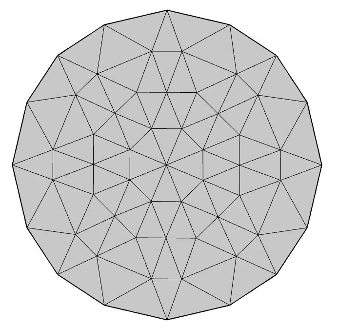
For mesh vertices on 3D surfaces, the Refine and Adapt operations place new vertices and moved vertices on a curved approximation of the surfaces. If you instead want a linear approximation, set the Face Representation setting to Linear. The figures below show how the new vertices that appear on the faces are placed on a curved or linear representation of the cylindrical faces. Note that for the linear representation, the geometrical edges of the top and bottom circles are still refined using spline curves.
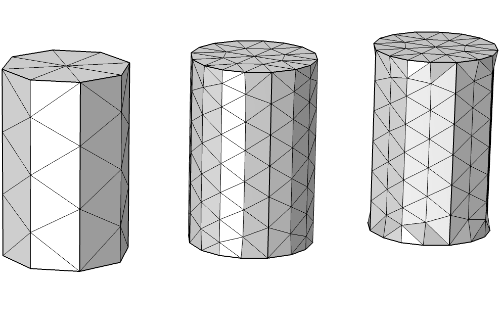
Adapting the mesh of a cylinder (left). The positions of the new mesh vertices on the faces and edges of the adapted meshes are determined by the Face Representation setting. It is set to Curved for the mesh in the middle and Linear for the one on the right.
Concluding Thoughts
We have shown how the Refine and Adapt operations can be used to modify and improve your imported meshes. Refine offers a quick way to easily decrease the size of your mesh elements, while Adapt allows for more granularity by specifying a Size expression. The General modification is especially powerful, as it is able to refine and coarsen the mesh as well as move vertices, thereby creating more isotropic elements and increasing the quality of the mesh.
Next Steps
The Adapt operation has a lot of useful features. If you would like to learn more about using Adapt and adaptive mesh refinement in the solver, try out these tutorial models:
- Parameter Optimization of a Tesla Microvalve
- Stresses in a Pulley
- 3D Super Sonic Flow in a Channel with a Bump
NASTRAN is a registered trademark of NASA.





Comments (0)