How to Use the Parameter Estimation Study Step for Inverse Modeling

When creating a simulation, you usually start by building the forward model, supplying various inputs, and then looking at the results. However, what if you have a set of results and want to find the input values that provide the same outcome? Here, we show how to use the Parameter Estimation study step, which helps you build an inverse model and solve for the optimal values of your model inputs.

Tutorial Video: Performing a Parameter Estimation Study in COMSOL Multiphysics®

Using the Parameter Estimation Study Step for Inverse Modeling

Suppose that you have a set of external data (either from experimental measurements or a collection of reference data) that you want to model your simulation after. In this situation, you can use inverse modeling. As the name implies, inverse modeling is when you take a reverse modeling approach to your problem: Instead of solving for the outcome, you solve for the inputs.

To get the desired simulation results, there are several model inputs that you might want to investigate or experiment with, such as material properties. When solving for the values of these inputs, you are looking for the optimal values that provide you with the closest match between a set of external data and the simulation results. A natural approach is to minimize the sum of the squares of the differences between the data sets. As such, an efficient modeling strategy is to formulate the problem as a least-squares optimization problem. To streamline the process of setting up and solving the problem, you can use the Parameter Estimation study step in the COMSOL Multiphysics® software.

To use the Parameter Estimation study step, the study must be time dependent and a license for the Optimization Module is required. In addition, a set of reference data needs to be included through either an interpolation function or user-defined reference expression. Note that the reference data must either be time dependent or a function of a single argument.

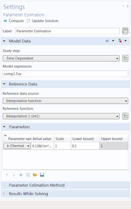
The Settings window for the Parameter Estimation study step.

The Parameter Estimation study step is useful for a variety of inverse modeling problems — mainly parameter estimation. The objective is to estimate values for the desired model inputs (i.e., parameters), which provides insight into the ways that the values (and hence the properties themselves) affect the objective function.

Perhaps one of the most typical uses of this functionality is curve fitting or similar data-fitting applications. This process involves fitting a function to a series of data points. The fitting of the function is done by estimating the values for the coefficients used in the function, essentially fitting a parameterized analytic function to a collection of data. By fitting a curve to a set of data points, we can interpolate values from the function to areas where data isn’t explicitly available.

In the tutorial video at the top of this blog post, we demonstrate a parameter estimation via a modified version of the elbow bracket tutorial model. Before computing this study, we need to properly define the problem…

Performing a Parameter Estimation Study in COMSOL Multiphysics®

Performing a parameter estimation study generally involves three major steps:

1. Prestudy: preparing the definitions, such as the parameters, variables, and functions
2. Study setup: customizing various aspects of the study and computing it
3. Poststudy: postprocessing to visualize and compare the simulation and experimental results, as well as extracting the optimal values for the estimated model inputs

Let’s look at how to complete these steps and the important factors to consider when setting up the Parameter Estimation study step in a model.

Step 1: Preparing Definitions for a Parameter Estimation

Before we perform a parameter estimation study, we must create the definitions needed to formulate the problem. This typically involves creating a combination of parameters, functions, and variables. First, we define the parameters of the model inputs for which we want an estimated value. Next, we include the external data by defining either a reference function or expression. Lastly, we define a variable that pulls and evaluates the output quantity from the simulation results, which are compared to the measured output data.

In the video above, we perform a time-dependent heat transfer analysis on the elbow bracket. The model data from the heat transfer simulation is then compared to the experimental data, which is used to estimate the value for the thermal conductivity of the material.

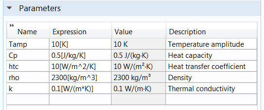
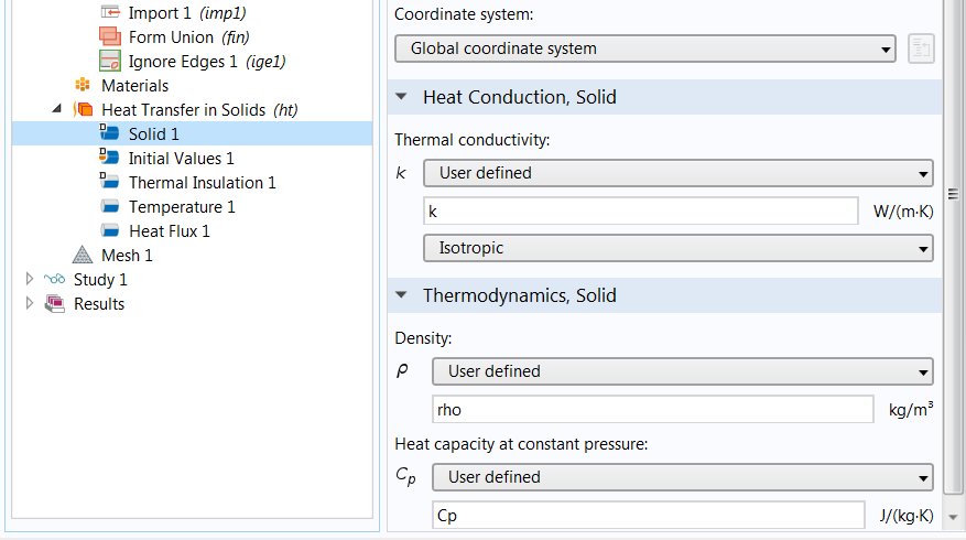
In the Heat Transfer in Solids node, the thermal conductivity is represented by k. Hence, we create a parameter named k, enter a rough estimate of its value, and use it in the appropriate node to define the thermal conductivity.

Left: The parameters used in the parameter estimation study, including the parameter k for estimating the thermal conductivity. Right: The node (named Solid 1) in which we use the parameter k to define the material property to be estimated.

Next, we create a definition so that we can implement the data from our external file into the COMSOL® software. In this case, the reference data is a collection of time-dependent temperature measurements contained in a comma-separated values (CSV) file. This data can be quickly and easily entered into COMSOL Multiphysics by adding an Interpolation function to our model component and then using the Load from File button. The data is automatically imported in a tabular format, with the first column containing the times and the second column containing the temperature measurements.

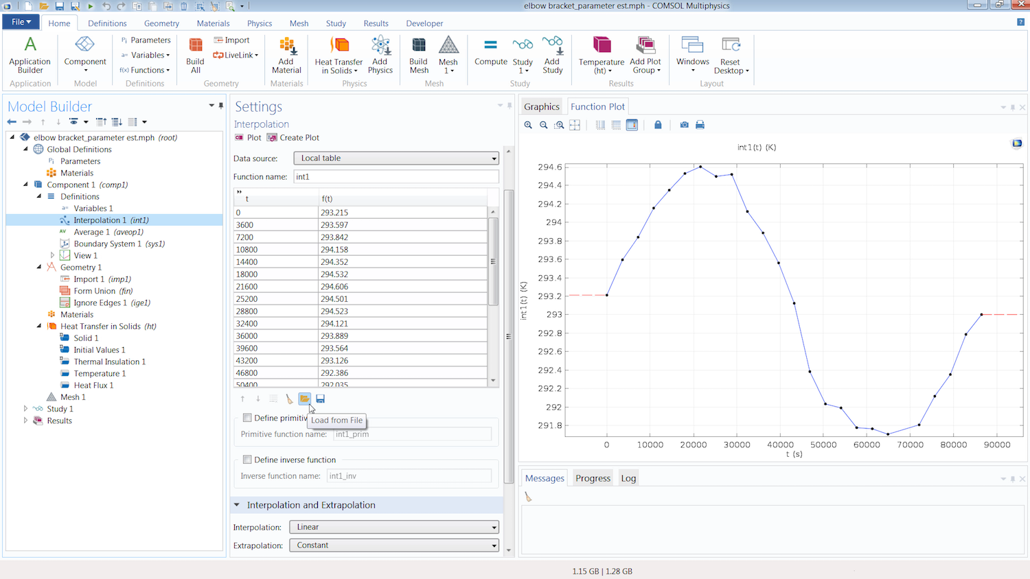
The Interpolation function incorporates the reference data into the simulation. The Load from File button is used to import the external file into the function.

Under the Units section, we simply enter the respective units for the argument (time) and function (temperature). We do not need to be concerned with the options selected for the Interpolation and Extrapolation settings of the function, since the study only computes the differences at the times explicitly stated in the argument or t column of the function. Thus, the smoothing between data points and the behavior of the function outside of the range of the data is not relevant.

We now need to define an expression to extract the temperature quantity from the simulation results. (This quantity is later compared to the temperature measurements in the interpolation function.) The quantity we want to extract and use for comparison is the average temperature of the surface on the top-right end of the bracket.

Since we want to obtain the average of a quantity (temperature), we first add an Average component coupling under the Definitions node. We then select the geometry we want to obtain the average temperature for (i.e., the boundary on the top-right end of the elbow bracket). Note the tag in parentheses to the right of the Average component coupling, aveop1, as this will be used in the expression for defining our variable.

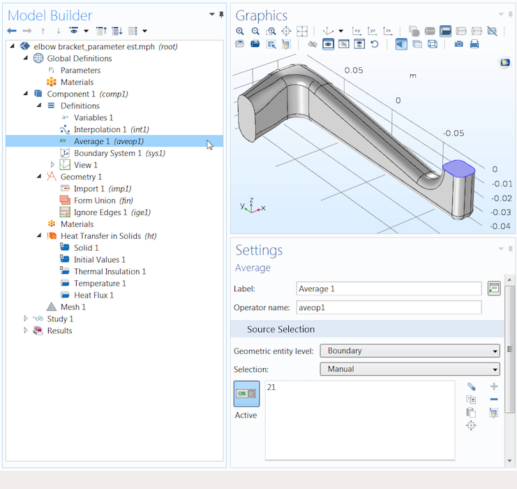
The Average component coupling (highlighted in blue) helps us obtain the average value of a quantity on the selected geometry.

To compare the computational and experimental results, we must define a variable to extract the quantity, and thus its value when computed, from the simulation results. Since we are looking at a specific part of the geometry, we define a local variable under the Definitions node or the Definitions ribbon tab. (A global variable is not suitable for our study, as the Global Definitions node is global in scope and defines, applies, or evaluates an expression over the entire model geometry.)

When defining the variable, we name it Tave, since we are looking to obtain the average (ave) temperature (T). For the expression, we can call out to the Average component coupling created earlier by entering aveop1. We then specify the quantity that we want the average of by entering the variable T (for temperature) in parentheses.

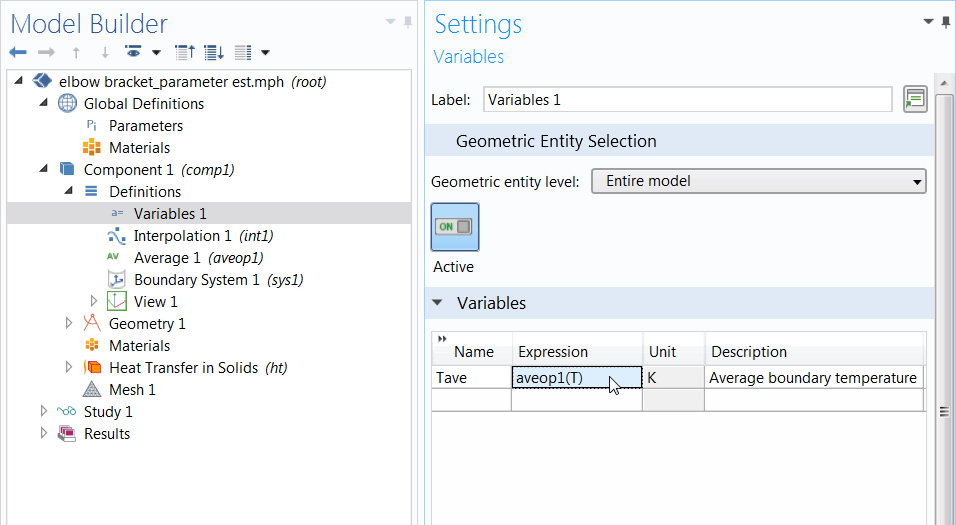
The defined variable, which is later used in the Parameter Estimation study step.

Step 2: Setting Up and Computing the Study

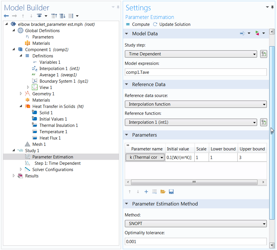
Now we can add and set up the Parameter Estimation study step, for which several settings have already been handled. The reference data and study step selections are automatically linked to the interpolation function that contains the external data and the time-dependent study.

The expression entered in the Model expression field is evaluated and then compared to the external data at each time step specified in the reference function; i.e., each time in the argument column of the interpolation function. As such, this field is where we enter our local variable, Tave.

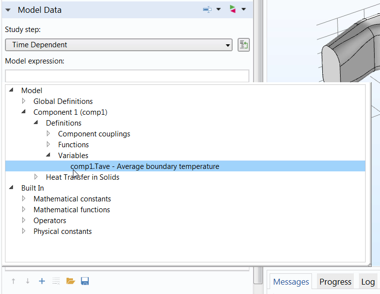
Notice that in the syntax of the Model expression field in the images below, we specify the location of our local variable, component 1, by including it before the variable name. The reason is that the scope of the Parameter Estimation study step is global. As a result, the study step does not “see” variables defined locally within a component unless we indicate their scope in the expression. For a global variable, we simply enter its name in the Model expression field. To enter the variable with its scope specified automatically, you can use the Auto Completion feature to select and enter the variable from the list of definitions.

Left: Using the Auto Completion feature to select the local variable defined earlier. Right: A screenshot of the completed setup for the Parameter Estimation study step.

Now we just need to identify the parameters we want to estimate and select the optimization method. We provide a rough estimate for the parameter under the Initial value column, add an upper and lower bound for the values that the parameter can take, and set the Scale value. Applying the appropriate scale is important, as it can significantly slow down the convergence of the optimization solver or stop it from converging altogether. Using the default value works for the elbow bracket example, but it might not always be suitable. (For more information, read the chapter on parameter estimation in the Optimization Module User’s Guide.)

Next, we want to select the appropriate optimization algorithm and compute it. The different methods apply to certain use cases, which are discussed in further detail in the video. Since the parameter we want to estimate controls the value of a material property — and we want to impose an upper and lower bound on the value — we use the SNOPT method.

Step 3: Comparing Results and Extracting Input Values

Once the model finishes solving, we need to perform some additional postprocessing. We can visualize and compare the two sets of data by plotting the results, and then we can extract the optimal values for the estimated model inputs. To see and compare both sets of data on a single plot, we add a new 1D Plot Group and include two Global plots under it. One Global plot displays the simulation results, while the other displays the reference data.

Since our interpolation function is a collection of data points, we want it to appear as a point graph. To do so, we change the time selection of the data points so that they are only plotted at the times specified by the argument column of the function. Additionally, we adjust several of the settings in the Coloring and Style section to further distinguish the two sets of data.

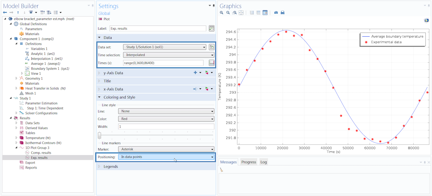
Comparison of the simulation and experimental results. The highlighted sections in the Settings window need to be adjusted to display the experimental data as a point graph.

This plot shows that the model results closely match the experimental data. We can now extract the optimal value for the thermal conductivity of the elbow bracket material. To do so, we add a Global Evaluation node under the Results tab (or under the Derived Values node). In the Settings window, all we need to do is update the Time selection option to Last so that we can evaluate the value in the last time step, since the thermal conductivity is independent of time.

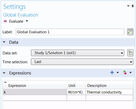
The Settings window for the Global Evaluation node.

After entering the parameter k in the Expression field, we click Evaluate and are provided with the optimal value for that parameter.

The optimal value for the thermal conductivity.

As shown above, a thermal conductivity of ~0.27 W/(m*K) provides the simulation temperature results that best match measurements from experimental data.

Modeling in Reverse via the Parameter Estimation Study Step

In COMSOL Multiphysics, the Parameter Estimation study step helps estimate the optimal values for the inputs of a simulation. By estimating the values that define various aspects of a model, you can investigate the parts of the problem that either hinder or help in best matching the computed results with a data set from an external file.

This functionality also enables you to solve other types of inverse modeling problems by streamlining and expediting the process of defining, setting up, and solving a least-squares optimization problem. For more details about this useful study step, watch the tutorial video at the top of this post, which provides guidance on how to use this functionality with a simple example.

Additional Resources

To learn more about parameter estimation in COMSOL Multiphysics, its use cases, and the various study step settings, read the chapters on parameter estimation in both the Introduction to the Optimization Module and Optimization Module User’s Guide documentation.

An archived webinar on parameter estimation is also available. (Note that the archived webinar uses the Optimization interface instead of the Parameter Estimation study step.)