Improving Convergence of Multiphysics Problems

In our previous blog entry, we introduced the Fully Coupled and the Segregated algorithms used for solving steady-state multiphysics problems in COMSOL. Here, we will examine techniques for accelerating the convergence of these two methods.

Load Ramping and Nonlinearity Ramping Techniques

As we just learned, the fully coupled approach to solving a steady-state nonlinear problem actually uses the exact same damped Newton-Raphson algorithm used to solve a single-physics nonlinear problem. Although this algorithm does converge well for many cases, it can fail or converge very slowly if the choice of initial conditions are poor. It should come as no surprise then that the techniques we have already looked at, such as Load Ramping and Nonlinearity Ramping, are just as valid when applied to a multiphysics problem. In fact, there is really nothing to add to these techniques — they can be used equivalently.

Ramping Multiphysics Problems

There is one new variation of the nonlinearity ramping technique, and that is to ramp the coupling between the physics. Numerically, it is in fact identical to the nonlinearity ramping technique already discussed, but conceptually it is the magnitude of the couplings between the physics that is ramped up, rather than the magnitude of the nonlinearity in a single physics. The only difficulty is choosing, and implementing, the term that should be ramped. Luckily, most multiphysics problems have quite obvious couplings between the physics, which can be found simply by writing out the governing equations and boundary conditions and examining how the material properties and loads are dependent upon the variables being solved for.

The most important thing to remember is that the underlying algorithm used to solve a fully coupled multiphysics problem is exactly the same as the algorithm used to solve a nonlinear single-physics problem. Keeping this in mind, you will find that fully coupled mutliphysics problems really do not pose any additional conceptual hurdles beyond understanding how the physics in the model interact with each other.

On the other hand, the segregated approach can lead to a variety of different solution strategies that can greatly accelerate solution convergence, and significantly affect the amount of memory needed to solve the problem. To understand this, let’s make a flowchart of the different multiphysics solution techniques. Consider the same problem from our previous blog post about a busbar that heats up due to current flow and experiences thermal stresses.

Fully Coupled Approach

First, the fully coupled solver starts from an initial guess and applies Newton-Raphson iterations until the solution has converged:

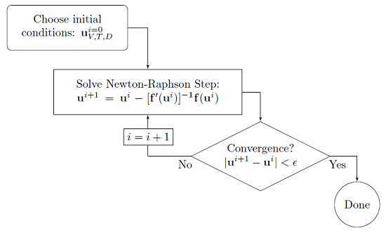
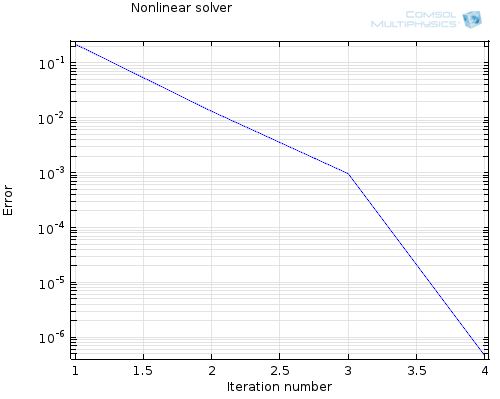
When solving such a problem, you will get a Convergence Plot, which shows the error estimate decreasing between Newton-Raphson iterations. Ideally, the error should go down monotonically if it does converge, then start investigating ramping the loads, the nonlinearities, or the multiphysics couplings. This approach will almost always require a more memory-intensive direct solver to solve the linear system of equations in each Newton-Raphson step.

Segregated Approach

Now, compare the fully coupled approach to the segregated approach, which solves each physics sequentially until convergence:

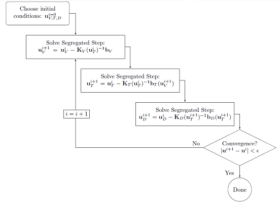
You will get a different kind of convergence plot for such a problem, one that shows the error associated with each physics you are solving. Each of the physics can use the optimal solver, either the direct or the less memory-intensive iterative, to solve the linear system of equations. Each segregated step can be a nonlinear problem on its own, and can be solved to a desired tolerance, and with custom damping, as appropriate for the particular combination of physics problem being solved.

With this solution method, you will get at least two convergence plots, one for the iterative solver(s) possibly used within a segregated step, and a second for the overall convergence of the segregated approach:

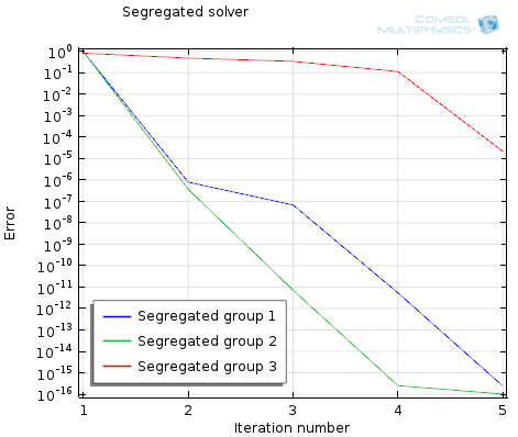
The above plot shows the decrease in error for each physics. Although more iterations may be required for the same problem, each loop through the segregated solution approach can be much faster than the Newton-Raphson step required for the fully coupled approach. You can also get a little bit more information out of this, if only one or two physics are not converging, then you will want to check the set-up of these first.

Sequential Solution Step

One thing you may recall about this problem is that the temperature change is driven by the resistive heating from the current, and the current distribution depends upon the electrical conductivity, which is temperature-dependent. That is, the voltage and temperature solutions are bi-directionally coupled. On the other hand, although the thermal strain and the Young’s Modulus are dependent upon temperature, the voltage and temperature solutions do not depend upon the displacements or stresses. That is, there is a uni-directional coupling from the thermal problem to the structural problem. We can immediately see that there is an even more efficient way to solve this problem. We can solve the voltage and temperature problem first and subsequently solve for the displacements:

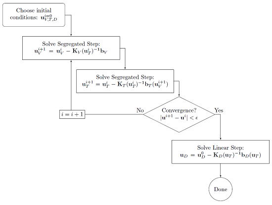
So, we can see that there are (at least) three different ways of solving this problem: fully coupled, segregated and assuming couplings between all of the physics are segregated, or with a sequential solution step to take advantage of the uni-directional coupling between temperature and displacements. When solving a multiphysics problem, COMSOL will assume coupling between all physics, and try to choose the optimal fully coupled or segregated approach, based on the physics and the problem size. Of course, it is always instructive to go into the solver settings to see what settings the software has chosen.

Conclusion of the Solver Blog Series

This series of postings has been designed to give you an understanding of the algorithms used in COMSOL to solve single-physics and multiphysics linear and nonlinear steady-state problems. Issues such as meshing, accuracy, and convergence have been covered. With this information, you should be able to more confidently address the solutions to your models of this type.