Introduction to Computing Radiative Heat Exchange

When modeling radiative heat transfer, we need to think about how radiation is emitted from a surface and absorbed by other surfaces, as well as how much radiation is exchanged between surfaces. We’ve addressed emission, reflection, and transmission in two previous blog posts in this series, and now we will finish learning the foundations of radiative heat transfer modeling by introducing the concept of view factors and the various ways to compute radiative heat transfer between surfaces.

This is the third blog post in a series on modeling radiative heat transfer. Read Part 1 and Part 2 here.

Quick Intro to View Factors

Let’s consider two thin, flat objects, as shown in the figure below. We will assume infrared radiation (IR) light can propagate freely in the space around these surfaces. This is true in a vacuum, and is reasonable for air and many other gases around room temperature. Cases when it may not be reasonable to assume unattenuated propagation include:

• IR absorptive gases, such as water vapor
• Gases at high temperature
• Gases with finely dispersed particulates
• Gases undergoing chemical reactions

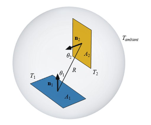
There will be radiative heat transfer between two isothermal objects at different temperatures. The objects can be thought of as sitting within an encapsulating ambient surface. The magnitude of the heat transfer is dependent on their size and orientation, and will occur only between the surfaces that are facing each other.

We will assume that these two objects are fixed at different temperatures. Outside of these two objects, there is nothing in our model of interest, but we also need to make one definition about all of the nonmodeled surrounding space. We need to define a uniform temperature, referred to as the ambient or background temperature. Although we will not explicitly model this ambient space, it is often convenient to imagine an encapsulating surface of fixed temperature.

Let’s consider the first object, and think about all of the radiation it emits. Some of the radiated heat flux goes toward the ambient, and some goes toward the second object. We now introduce the concept of the view factor, which is the fraction of radiation that leaves Surface 1 (A_1) and arrives at Surface 2 (A_2), and is written as F_{12}. Assuming uniform radiosity and that there are no intermediate obstructing surfaces, the view factor between these surfaces is:

When there are more than two surfaces in the system, it is possible that they can all see each other, so we write the view factor as F_{i j}, where i,j is the index of all of the N interacting surfaces of the model. Between any two surfaces, the reciprocity relation holds: A_i F_{i j} = A_j F_{ji}.

Note that if a surface is concave, then F_{i i} >0. It’s also worth remarking that the heat flux to ambient is defined via the ambient view factor: F_{i \rightarrow amb} = \left( 1 – \sum_{j=1}^N F_{ij}\right). For a closed cavity, the ambient view factor is zero.

Three Methods for Computing Radiative Heat Exchange

The three methods for computing radiative heat exchange are:

1. Direct area integration
2. Hemicube
3. Ray shooting

1. Direct Area Integration

The direct area integration method works by performing a double integral over all pairs of surfaces. It can be used as long as there are no obstructions or shadowing between the surfaces. This method has proved to be accurate, with the accuracy controlled solely by the radiation integration order.

The reciprocity relationship is always fulfilled with this method, but the ambient view factor might be different from zero for a closed cavity if too low of a discretization and a very coarse mesh are used. Direct area integration does become computationally intensive if there are many elements. Also, since shadowing is not considered, it is primarily useful for modeling small concave cavities, so in practice, it is used sparingly.

2. Hemicube

The hemicube method can be conceptually understood from the image below. Consider a single surface element, draw five boundaries about that element, and pixelate them uniformly. Then, project the surrounding faces onto these pixelated boundaries and count the pixels associated with each face to determine how much radiative heating is coming from the surrounding faces, and is irradiating that element. Repeat this for every surface.

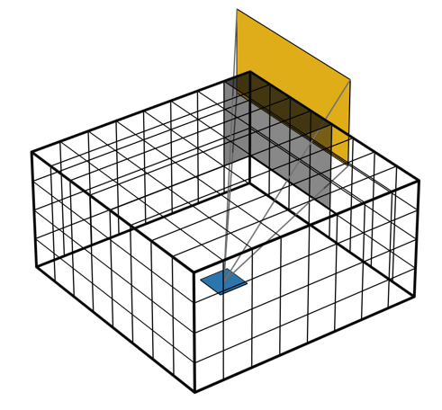
The hemicube method projects surrounding faces onto a set of pixelated boundaries to compute irradiance.

Shadowing of faces is treated efficiently by z-buffering, so the computational cost is low. The single setting for this method, Radiation Resolution, governs the number of pixels. The accuracy of the reciprocity relationship will improve with increasing radiation resolution, and the ambient view factor for a closed cavity will always be zero.

3. Ray Shooting

The ray-shooting method is useful for cases where there is angle-dependent emissivity, specular reflectivity, or semitransparency. The ray-shooting method, as its name implies, shoots rays in space. It is important to note, though, that this is a reverse ray-tracing method. From the evaluation point within each element, a set of rays are cast outward and used to determine the irradiance from that direction. So, think of the rays as going in the opposite direction from the incoming radiation. These rays represent a finite sampling of the total irradiance from the surrounding hemispherical space.

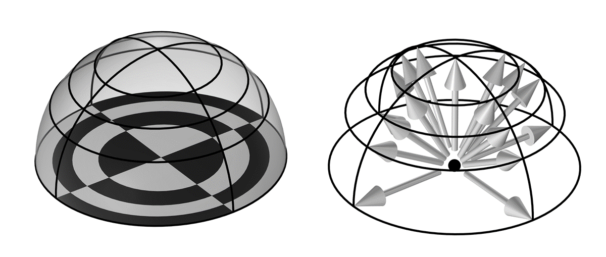
Illustration of the ray-shooting method in terms of the discretization of a 3D hemisphere, for a radiation resolution of 4. Each tile of the 16 tiles of the base checkerboard (left) has equal area. Arrows point toward the corner of each tile on the hemisphere (right).

The ray-shooting method has six settings that can be changed, as well as the element order. The most important of these to understand is the Radiation Resolution, which defines an initial distribution of rays over a hemisphere (in 3D) or half circle (in 2D), as shown in the image above for a radiation resolution of n_{res}=4.

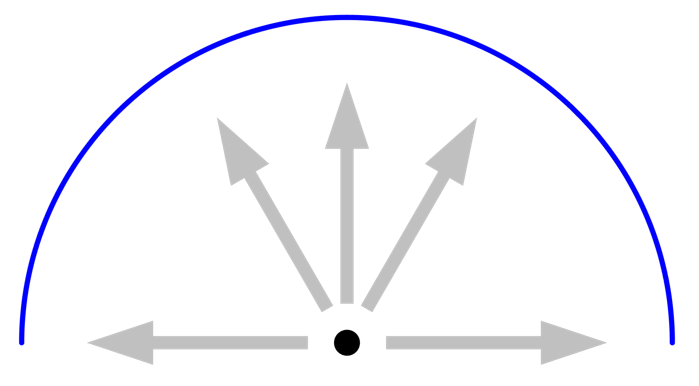
The method begins by subdividing the surroundings into n_{res}^2 number of tiles in 3D (or n_{res} in 2D) and then drawing a ray to the corner of each tile. Each of these tiles has the same view factor, meaning that, via the Nusselt analogy, the projected area of each tile onto the plane below is equal. For the 2D case of a half circle, as shown below, the surroundings are divided into n_{res} tiles, each having the same projected area onto the plane. Note how this leads to a nonuniform, angular distribution of rays, as illustrated below.

Illustration of the ray-shooting method for the 2D case. Each sector of the semicircle (left) has equal projected area onto the line below. Arrows point toward the corners of each tile (right).

When the ray is cast outward, it essentially queries the heat flux that is coming from that direction, and then compares it to the heat flux coming from the neighboring rays. If there is a difference in the flux, as defined by the Tolerance setting, then the ray-shooting method will start introducing additional rays in between, up to what is specified in the Maximum number of adaptations option. When the ray hits a specular reflective, or transmissive, surface, an additional ray is launched from that surface as well, up to the Maximal number of reflections. The default of 1000 is reasonable unless dealing with many reflections inside of a cavity with specular reflectivity greater than 0.99.

The Angular dependent properties setting is only applicable when there are surfaces with angular-dependent emissivity. The default Full resolution setting is not only the most accurate, but also the most computationally intensive, as compared to the Interpolation function option, where you can specify how finely to sample the angular dependence function.

It is primarily the Radiation resolution and Maximum number of adaptations that need to be studied to get confidence in the results, so it is important to understand the interplay between these settings. Let’s look at a 2D case and consider the rays being shot out from an element at the center. It should be remarked that this plot is a visualization only; the computational rays themselves are not plottable. We consider a surrounding half circle of unit emissivity (equivalent to zero reflectivity) and fixed uniform temperature, meaning that each ray sees the same radiative load. In this case, even the most minimal radiation resolution will give the correct answer for the flux. Higher resolution (more rays) will not lead to higher accuracy and no adaptation is ever triggered.

Next, let’s introduce a small object, also of unit emissivity but at different temperature, at an angular location that happens to coincide exactly with one of the ray directions. This ray will now see something different from its neighboring rays, and the angular space is subdivided, as illustrated below. Increasing the maximum number of adaptations will increase the accuracy, but there is no need to increase the ray resolution since the small object is already seen by one of the initial rays. This adaptation of rays will occur based on sensing a different irradiance from different rays, so it will also work if a single surface has a spatial variation of radiated flux.

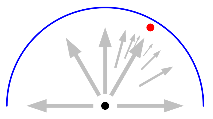
Introducing a small object that gets seen by one of the rays will lead to the adaptation of rays in the neighboring space. A higher number of adaptation will increase accuracy.

Finally, let’s introduce another small object at a different angular position that does not coincide with one of the initial radiation resolution directions. In this case, it does not matter what the maximum number of adaptations is. This second object is never “seen” by any of the initial rays. To see this second object, the radiation resolution has to be increased as well.

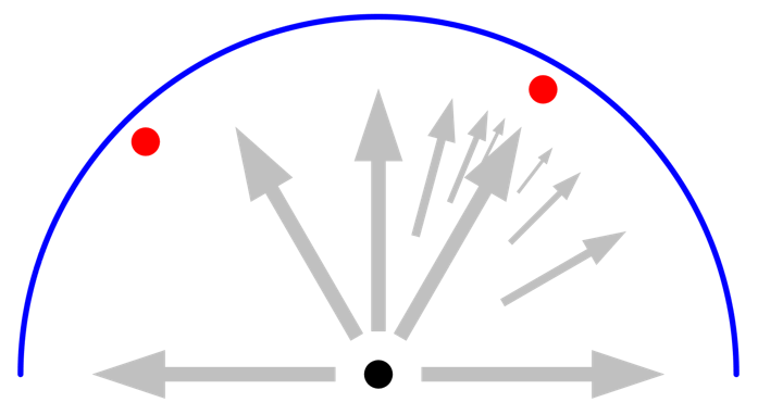
If a small object is not seen by one of the initial rays, as defined by the resolution, no adaptation is performed by the nearby rays, and it will be missed. This case requires increasing the radiation resolution.

Using Radiation Groups

In parallel with all of the abovementioned methods, it is possible to use so-called radiation groups. By selecting sets of boundaries that can only see each other — especially in a model with several distinct cavities — the computational cost is reduced. Groups must be used carefully, though, since they can produce erroneous results if the grouping is incorrect.

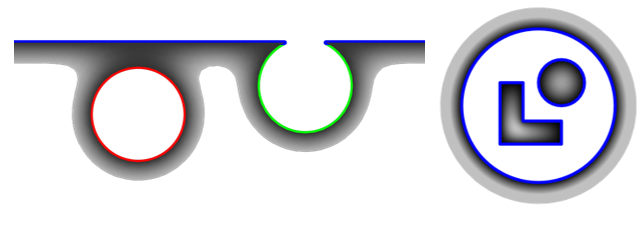
When a distinct set of surfaces cannot see others, it is reasonable to use the Groups functionality. On the left, different colors indicate a reasonable grouping. The case on the right is less amenable to using Groups.

Other Surface-to-Surface Settings

For models that include moving or deforming objects, it is necessary to update the view factors, as controlled by the View factors update threshold settings. The default of updating at every nonlinear iteration provides the most accurate results, but can be expensive. It is possible to turn off the view factor update entirely, which can make sense for an object that is moving or deforming in a way that has a negligible effect on the view factors. It is also possible to update periodically in time or via a user-defined expression.

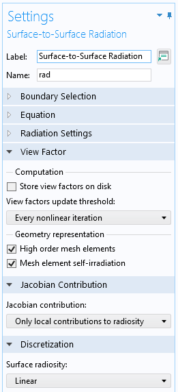
The View Factor settings of the Surface-to-Surface Radiation interface.

The View Factor settings also let you store view factors to disk. This can save time for larger models, but the size of the model file on disk will be substantially larger, especially with the Hemicube method. This setting should only be used if the geometry is not changing.

The Geometry Representation settings come into play if the geometry shape function is higher than linear. If you increase the discretization, these options will consider the curvature of the elements.

Finally, the Jacobian Contribution is, by default, set to Only local contributions to radiosity. This default setting, as of version 6.0 of the COMSOL Multiphysics® software, will lead to lower memory usage and faster solution times. However, it can fail if the model is purely radiatively cooled and has significant temperature variations between surfaces. If you observe nonconvergence, change this setting to Include contributions from total irradiation.

Evaluating and Plotting View Factors

If you have several sets of surfaces and want to know the view factors between them, this is addressed in a previous blog post. It is also sometimes helpful to plot out the view factor from one surface to all the other elements in the model. This can be achieved via the elemint(order,expression) operator, which performs a Gaussian integration over each element. The order of the integration is given by the first argument, and to evaluate the view factor, we use the radopu() and radopd() operators within the expression. For example, plotting the expression:

elemint(1,comp1.rad.radopu(S1,0))/intS1(1)/dvol

will evaluate to, on an element-by-element basis, the view factors from the set of surfaces defined by the integration operator intS1() to all other surfaces in the model.

The variable, S1, should be defined as 1 over the set of surfaces that is illuminating and zero on all illuminated surfaces. An example of this type of plot is shown below. By additionally dividing the size of the illuminated element, the variable dvol, we get a plot that corresponds to the illumination intensity from one set of surfaces, as shown below.

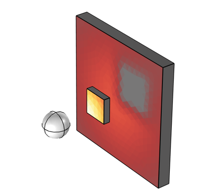
Visualization corresponding to the illumination from a sphere to two blocks that partially shadow each other.

Closing Remarks

We have now looked at the three key conceptual components of modeling radiative heat transfer between surfaces surrounded by a nonparticipating medium. First, we looked at the different ways in which a hot surface can emit thermal radiation. Next, we looked at how radiation incident on a surface can be absorbed, reflected, and transmitted. Finally, we’ve addressed view factors and how to compute and update them. With these pieces in place, we are now ready to tackle thermal radiation with confidence!