
In engineering analysis, the need to compare solutions obtained under different circumstances frequently arises. Some possible scenarios include comparing the effect of different load or parameter configurations, and enveloping results to find the worst or best case at each point of the domain. In each of these and other similar cases, you need access to more than one data set. Here’s how to accomplish such tasks using COMSOL Multiphysics.
The Join Feature in COMSOL Multiphysics
To join solutions, right-click on Data Sets under “Results” and choose Join. When using the ribbon (or menu if you’re running Mac® OS or Linux®), the command is Results > More Data Sets > Base Data Sets > Join. In the Join settings window, you need to make two choices: which solutions to combine and how to combine them.
You determine the base data sets under the Data 1 and Data 2 sections. Right beneath Data 2, you can configure the combination method.
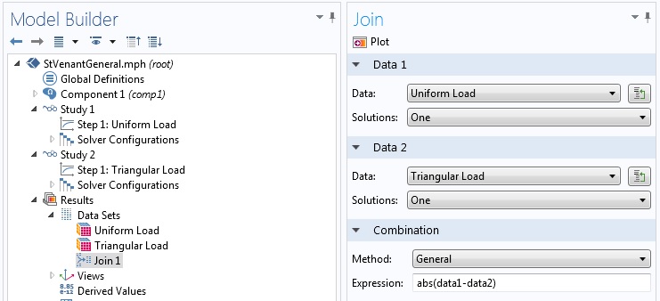
The Join settings window.
There are seven choices for the combination method. However, five of those can be taken as special cases of the other two options. We will start by discussing the General and Explicit methods.
General Joining
When Method is set to General, a field appears where you can enter an expression. For instance, data1-data2 makes a difference expression and (data1-data2)^2 the square of a difference. The latter can be used, for example, as an integrand for evaluating difference in the L2 norm.
At this stage, the variable that is going to be compared is not specified. In essence, we are constructing an operator that can later be used with any quantity defined in both of the original base solutions. Consider a problem where T is the dependent variable, such as in a heat transfer problem.
Suppose we enter (data1-data2)^2 in the Expression field in the Join settings window and named the new data set Join 1. Then, to plot the square of the difference in the temperature, we choose Join 1 for Data set and T for Expression in the plot settings window.
To demonstrate the use of solution joining using the General method, we will consider two modeling examples.
Example 1: Absolute Difference
In this example, a 2D plane stress model of a membrane with a thickness of 0.1 meters is alternately loaded by a uniformly distributed load of 10 MN/m along the right end and a triangular load at the same edge with a maximum intensity of 20 MN/m at the center and vanishing at the ends. These two loads are statically equivalent. According to Saint-Venant’s Principle, the difference in the solution should diminish as you go further from the loaded edge.
We compute two stationary solutions using first the uniform load and then the triangular load. Then, we create a joint solution Join 1 using the General combination with abs(data1-data2) in the Expression field as shown in the above figure. To plot the absolute difference in the von Mises stress, we now make a surface plot using the Join 1 data set and solid.mises in the Expression field of the Surface settings window. In the figure below, the difference is large near the loaded edge and much smaller far from the edge, as predicted by Saint-Venant’s Principle.
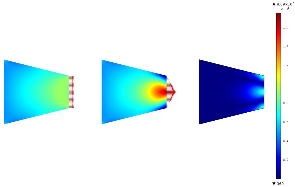
Von Mises stress with uniform and triangular edge loading, and absolute difference in von Mises Stress.
Example 2: Result Enveloping
Engineers run analyses for different conditions and want to know the best or worst case situation at all points in the domain. For example, in a thermal analysis, the maximum temperature is of interest. At some points in the domain, the maximum temperature is encountered for one set of boundary or domain conditions and at other points for other sets of conditions. The temperature envelop shows the extreme temperature values at each point under any circumstance.
In this example, we consider a simple stationary 1D heat conduction problem. In the first case, the temperature goes from 300 K at the left end to 400 K at the right end. In the second case, the temperature is flipped, going from 400 K at the left end to 300 K at the right end.
To construct the maximum temperature envelop, we make a joint data set Join 1 from the two solutions using the General method and max(data1,data2) for the expression. Then, in a line plot, we choose Join 1 for the data set and T for the expression to get the maximum temperature envelop (depicted below).
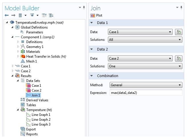
Result enveloping settings.
In the plot below, you can see the joining operation and the result envelop together with the results from the two base cases:
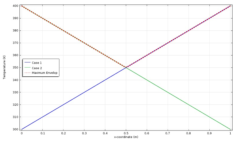
If we want to plot the minimum temperature envelop, we have to add a new joint data set using min(data1,data2) in the Join settings window.
Explicit Joining
There is one restriction when using the General method for joining: you have to use the same variable from both base solutions in subsequent operations, such as plotting or integration. For example, to plot the sum of the variable u from the first data set and the variable v from the second data set, you cannot use the General method. If we have data1 + data2 under Expression in the Join settings window, we can use it either with u, which returns data1(u) + data2(u), or with v, which returns data1(v) + data2(v).
This is where the Explicit method comes in handy. When you opt for this method, COMSOL Multiphysics makes two new operators, data1 and data2, which can be used to access quantities from the first and second data set, respectively. A difference with the General method is that there is no field for typing an expression at the solution joining stage. The two operators can be used directly later in the plot, integration, average, or other settings. For instance, data1(u) + data2(v) can be typed in a plot settings window, provided that u is a legitimate variable in the first solution and v is available in the second solution.
Another advantage of the Explicit method is that since an expression is not fixed at the solution joining stage, you do not need to create a new joint data set to use a different expression. In a 1D heat transfer problem, for example, we can make an Explicit joining and use it in two different line integrations for both the L2 and H1 norms. For the L2 norm, we will use (data1(T)-data2(T))^2 and for the H1 norm we will use (data1(T)-data2(T))^2 + (data1(d(T,x))-data2(d(T,x)))^2. Here, d(T,x) is the derivative of T with respect to x, which is a predefined operator in COMSOL Multiphysics.
Going back to the temperature envelop example, we needed two joint data sets to make the maximum and minimum temperature envelops using the General method. If we instead went with the Explicit method, we would only need one joint data set and use max(data1(T),data2(T)) and min(data1(T),data2(T)) in line graphs to plot the maximum and minimum envelop, respectively.
Using Operators on Joined Data Sets
General Method
You may add functions and component coupling operators in the Definitions node of the Model Builder. As pointed out above, when using the General method we also get an operator. Thus, we end up with a composition operator when we employ a user-defined coupling operator or function with a data set joined using the General method. The question is: Which operator is the inner operator and which is the outer operator in the composition? The answer is that the operator made by the solution joining is the outer one and any operator added in the Definitions node becomes the inner operator. Let us look at an example to illustrate the idea.
Consider a coupling operator intop1 added in the Definitions node of the above 1D heat conduction example. A data set Join 2 is made from two solutions using the General method and the expression (data1 - data2)^2. If we choose Join 2 for Data set and intop1(T) for Expression in Results > Derived Values > Global Evaluation, will we get the L2-norm of the difference between the two base solutions? The answer is no. The global evaluation returns a value of zero.
Since intop1 is the inner operator, what gets evaluated is (intop1(T)-intop2(T))^2, which clearly is not the L2 norm of the difference. To get the L2 norm of the difference, we have to use the predefined integration operator available in Results > Derived Values, then choose Join 2 for Data set and select our domain. Finally, use T for Expression. The figures below show the COMSOL Multiphysics implementations of these operations and their mathematical representations.
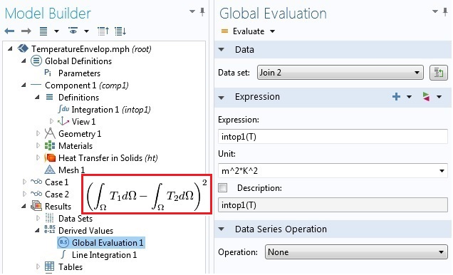
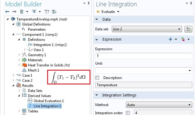
Using operators on joined solutions with the General method.
In summary, the order of operators in a composition operation is as follows: functions or coupling operators added in the Definitions node; the operator created by Join; and predefined average, maximum, minimum, and integration operators available in Results > Derived Values, from inside to outside.
Explicit Method
When using the Explicit combination, the situation is clearer. The figures below show how the difference of the integrals and the integral of the difference are evaluated on an explicitly joined data set Join 3.
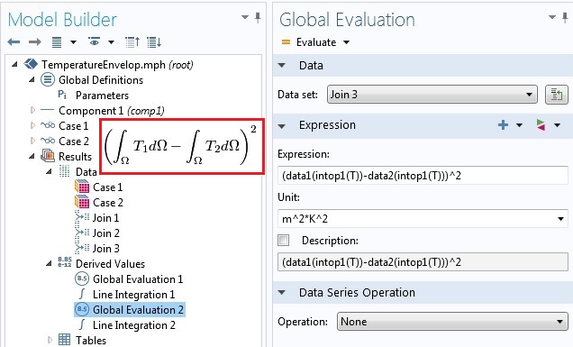
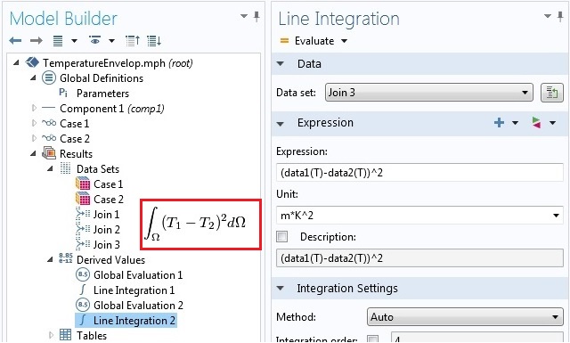
Using operators on joined solutions with the Explicit method.
Other Joining Methods
The other five combination methods are Difference, Norm of Difference, Product, Quotient, and Sum. They are equivalent to using the General method with data1-data2, abs(data1-data2), data1*data2, data1/data2 and data1 + data2 for Expression. Of course, whatever can be done with the General method can also be done with the Explicit method by building the expression later at the point of use.
In this blog post we have focused on joining stationary solutions with no parametric sweeps. In the case of parametric sweeps or in time dependent solutions, each base solution contains more than one data set. The same is true for eigenfrequency and frequency domain studies. For these study types, solution joining can be used to evaluate some useful and interesting quantities. We discuss that in a follow-up blog entry.
Need More Help?
- Browse the Support Center
- Contact us


Comments (11)
Thales
July 1, 2014Very good post!
We users want posts like this!
Maybe in further posts it could be mentioned more clearly the operators “at” and “with”, it was briefly mentioned in a previous post, but without much emphasis. For example, if you have a parametric sweep with 2 variables, it’s cumbersome to compare different stages with “with”, in matlab it’s simpler.
Anyways, thanks for the post.
Hossein Mousavi
August 5, 2014I really like the new COMSOL capability to join two separate solutions into one dataset using the Join functionality.
However, it seems the data2 special operator returns only the real part of its argument, only it is the data1 operator that can handle both components. Is that a bug or is that meant to be?
For example, imag(data2(u)) is always zero.
Nikita Kondratiev
August 6, 2014Looks like there are a lot of bugs here:
with() operator doesn’t work with data2
intop3(data2(u)) gives out an error
“surface integration” and “global evaluation”(intop()) give different results
The worst is that you can’t join two data sets of eigenvalue problem solutions (probably any data sets with more than one solution):
if you try to join both with all solutions it just gives out an error
if you join first dataset with “all” and the second one with “one”, you can’t get to other solutions from second dataset
if you join first dataset with “one” and the second one with “all”, Comsol gives out errors while making tables
It is a pity that it also can not join more then two datasets (for example in nonlinear physics you may need to calculate something like intop(u*v*h*…), where u, v, h, … are solutions of different eigenvalue problems)
At the end it looks like this feature brings no new functional, duplicating the one given by study steps.
However it is a first node, allowing manipulation with data sets. I hope the developers will improve it to work as desired. More functions (like one collecting only desired solutions from all in dataset or removing unnecessary) will be appreciated.
Temesgen Kindo
August 6, 2014Hello Hossein,
Thanks for the comments.
In the explicit joining when you are using operators the right syntax is datan(operator(variable)). In your case it should be data2(imag(u)).
Temesgen Kindo
August 6, 2014Dear Nikita,
Thanks for the feedback. I will try to address some of the issues below.
1. When you want to use an operator with an explicitly joined data set, the correct syntax is data(operator(variable)). In your case that become data2(intop3(u)).
2. The surface integration and the global evaluation give different results because we are evaluating different expressions. This is not a bug. It is deliberate. If you see the mathematical expressions in the red boxes, they are different quantities. Which one you want to use depends on what you are doing. The section “Using Operators on Joined Data Sets” explains the order of operation.
3. You can work with solutions corresponding to more than two eigenvalues. One option is to use the built-in WITH operator. Another option is to first join two data sets and then joined that joined data set with a third solution. Please see the follow up entry here for more. http://www.comsol.com/blogs/solution-joining-parametric-eigenfrequency-time-dependent-problems/
4. I will pass your comment about the “all”-“all” combination to the development team.
Hopefully this addresses most of your items.
Thank you again.
Nikita Kondratiev
August 7, 2014Dear Temesgen,
Thanks for your clarification. It helped a lot. However some points are still unclear.
1. Yes, that works! Thank you very much!
The funny thing is that data2(with(n,u)) works even if you have chosen only one solution to join.
2. No, you misunderstood me. I do exactly “global”->data1(intop3(with(1,u))) and “Surface”->data1(with(1,u)), which should give out the same, but it does not. Actually, I found the issue today.
The problem was in automatic selection determination for joins in surface integration. While I can input it explicitly for “intop” and surface integration of ordinary data, I do not get that dialog for joined data set.
3. The WITH operator works only within one solution, so I have to use join if I need to combine different modes from three different data sets.
For example for 4-order non linearity I have 4 data sets of, say 1000 modes each. So I have to make a join of first pair of sets, choosing manually two of 2000 modes. Then I make another join with the third data set, choosing one mode and finally the last join with the whole last set. Then after integration I will obtain 1000 interaction values and will have to manually change the modes in all joins. Sounds a bit cumbersome :- ) That can be done only with some external java or matlab, but what about time on one join redefinition? The construction data1(data1(data2(with(n,u)))) also does not look time-optimized. Although it works.
4. “all”-”all” combination should probably work like multiparameter sweep, producing, as you call it, vectorized list of the parameters.
The whole construction also lacks “conditional” solution selection (apart from “manual” and “from list”, that are everywhere except join), which could choose solutions according to some evaluation.
Aleksandr Spiridonov
September 21, 2017Temesgen,
Thanks for the article. Good stuff!
You do need to add a paragraph to address integration of explicitly joined data sets in the axisymmetric case:
By default, when the “Compute volume integral” is checked (assuming it’s a 2D axisymmetric study and you’re integrating over a surface) trying to do the integral will cause an error, shown below, since the “r” coordinate does not exist in the Join data set and only in the data1() and data2() sets. To address this, we have to manually multiply the expression by “pi * data1(r)” to get the volume integral.
Reference error:
”
Undefined variable.
– Variable: r
– Global scope
Failed to evaluate expression.
– Expression: 2*r*sqrt(((data1_join1_join1_2__re+i*data1_join1_join1_2__im)*(data2_join1_join1_1__re+i*data2_join1_join1_1__im))^2+((data1_join1_join1_1__re+i*data1_join1_join1_1__im)*(data2_join1_join1_0__re+i*data2_join1_join1_0__im))^2)*pi^2*(data1_join1_join1_0__re+i*data1_join1_join1_0__im)
”
Keep up the good work!
Alek
Abdallah EL SOUSSI
January 26, 2018Hello,
If i have two solutions, one for optical modes and the other for accostical modes, at first i was intrested in doing surface integration with one optical mode and one accoustical mode so i used the join data option but now i am intrested in two optical modes and one accoustical mode so jow can i join 3 data solutions please?
Temesgen Kindo
January 26, 2018Dear Abdallah,
You have a couple of options here.
Option 1: Joint the first two data sets. Then that data set now becomes available for another joining operation with the third data set.
Option 2: Using the with and withsol operators. Please see the COMSOL Reference Manual for details on these operators.
If you encounter difficulty implementing these options, please contact COMSOL Technical Support.
Best Regards,
Temesgen
Sergey Kuznetsov
February 22, 2021Hello!
How do I stitch solutions from two time dependent steps?
Debadutta Mohanty
January 1, 2025how to make vaccum surface in inside a double rectangular geometry (inner rectangular )