Maximum Evaluations on Parallel Sections

In a previous blog entry, we shared a postprocessing technique for creating an animation by combining parallel slices in a 3D steady-state model. Today, we will look at another postprocessing trick: how to evaluate and plot the maximum (or the minimum, average, or integration) value of any variable at various parallel sections along the axial coordinate.

Postprocessing Objective

Any field variable u = u(x,y,z) in a 3D model could have a different maximum value in various xy planes, i.e., (u_max)_i at z_i and (u_max)_i+1 at z_i+1, as shown in the plot below. Our objective is to generate a plot for the field maximum (u_max)_i, which is the field maximum at the i^th plane along the axial direction. There are multiple ways to address this postprocessing question.

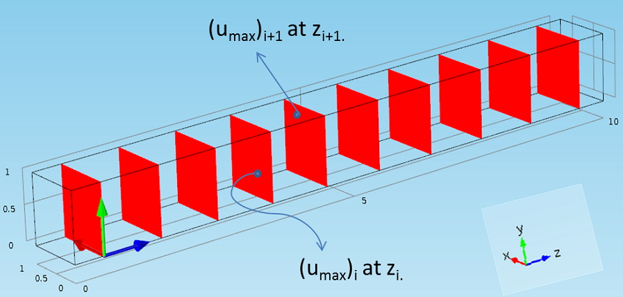
A schematic showing different field maximum values on parallel sections.

A Cut Plane Data Set

The first approach would be to use the built-in postprocessing features such as the Cut Plane data set and the Surface Maximum feature. You could create a Cut Plane data set at a particular z-location. The maximum value of any variable at this plane can be evaluated using the Surface Maximum feature (under Derived Values > Maximum > Surface Maximum). With this approach, the cross-sectional maximum can be evaluated at a single z-location. This procedure must be repeated for different axial locations to obtain maximum values at each of these cross sections.

LiveLink™ for MATLAB®

The manual procedure outlined in the above section can be automated using LiveLink™ for MATLAB® through a simple ‘for’ loop. The built-in wrapper function ‘mphmax’ enables the maximum calculation for a Cut Plane data set. Here is the sample code for evaluating the maximum cross-sectional values (u_max vector with ‘n’ values) for z = [z₁, z₂, …, z_n] given that the Cut Plane data set is already defined in the model:

z = [z1 z2 z3   zn];

for i = 1:length(z)

  model.result.dataset('cpl1').set('quickz', z(i));

  umax(i) = mphmax(model,'u',2,'dataset','cpl1');

end

plot(z, umax)

The Parametric and Auxiliary Sweep Features

The Parametric Sweep or Auxiliary Sweep features are available to run COMSOL Multiphysics models for multiple values of any given parameter (used for defining geometry, mesh, and physics settings). Because these sweep features are essentially a ‘for’ loop, we can even utilize the features for a postprocessing analysis such as this.

Let’s look at the various steps needed to create the cross-sectional maximum value plot for the velocity magnitude in the Laminar Static Mixer model. The slice plot below shows the velocity field magnitude at various z-locations. Our objective is to obtain the maximum velocity magnitude on each of these slices (cross sections) and plot these slice maxima with respect to the z-coordinate.

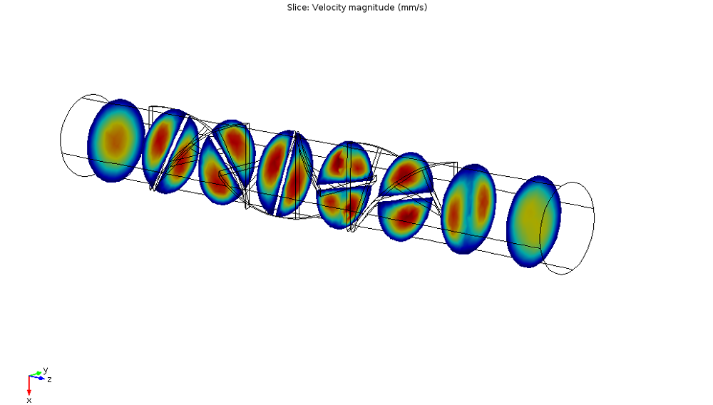
Velocity slice plot for the Laminar Static Mixer model.

Step 1

The first step is to add a parameter corresponding to the axial coordinate. For this example model, we add a parameter zp, as shown in the screenshot below.

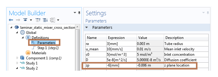
Adding a parameter in the Parameters table.

Step 2

Next, we need to add a second study (with a stationary step) to run the Auxiliary/Parametric sweep with respect to the parameter zp. The sole purpose of using the second study step is to restructure the available solution data in order to achieve our postprocessing objective. Therefore, in this step, we do not solve for any physics interfaces and simply pass along the solution from Study 1 to this study.

Using the Stationary step settings mentioned above (and also noted in the snapshot below), we then need to compute the second study step.

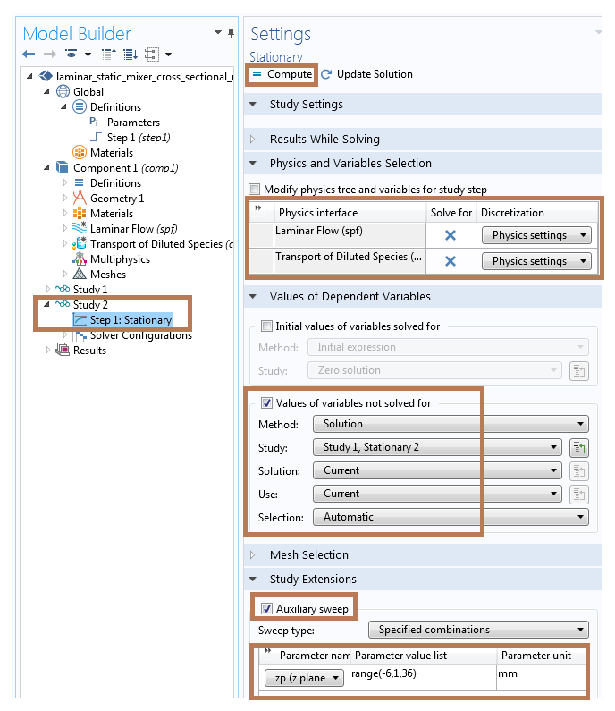
Stationary step settings for running the Auxiliary Sweep feature without solving for physics interfaces.

Step 3

We now need to add a Parameterized Surface data set (right-click on Data Sets under the Results node and select “Parameterized Surface” from the More Data Sets submenu). In the Parameterized Surface settings, we will use Study 2/Solution 1 as the data set and parameter zp as the z-coordinate expression. This is illustrated in the image below.

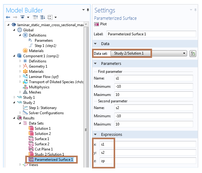
Settings for creating the Parameterized Surface data set.

Step 4

In the next step, we need to add a Surface Maximum node to the model (right-click on Derived Values under the Results node and choose “Surface Maximum” from the Maximum submenu). We utilize the Parameterized Surface as the data set for evaluating the Surface Maximum, as shown in the Surface Maximum settings below. Now, click on Evaluate to create a table with plane maximum values (velocity magnitude) for each of the z-coordinate values.

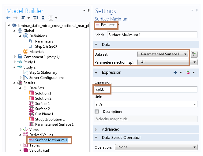
Settings for evaluating the Surface Maximum using the Parameterized Surface data set.

Step 5

Lastly, we can click on the Table Graph button (shown in the figure below) to plot the table data. The 1D plot indicates the maximum velocity field magnitude plotted versus the z-coordinate location.

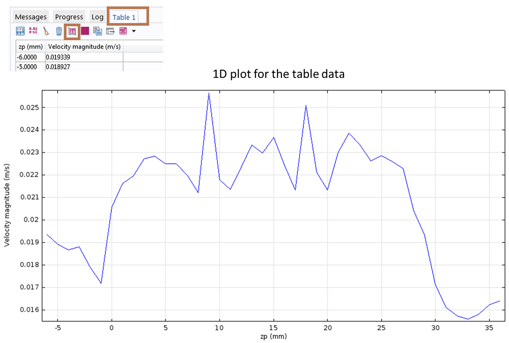
1D plot showing the cross-sectional maximum values for the velocity field magnitude at different z-coordinates.

Summary

This post demonstrates a very simple — yet powerful — postprocessing trick for automating the maximum (or the minimum, average, or integration) calculation for any variable on parallel planes. The key concept we have highlighted here is how to use the sweep functionality within COMSOL Multiphysics to restructure the available solution data for postprocessing purposes. We have also presented a scripting solution using LiveLink™ for MATLAB® that would require only a few lines of code in order to complete this postprocessing task.

Stay tuned for the next entry in this blog series for additional tips and tricks!

MATLAB is a registered trademark of The MathWorks, Inc. All other trademarks are the property of their respective owners. For a list of such trademark owners, see http://www.comsol.com/tm. COMSOL AB and its subsidiaries and products are not affiliated with, endorsed by, sponsored by, or supported by these trademark owners.