
Want a roadmap to modeling cables? We have an eight-part tutorial series for you. The Cable Tutorial Series shows how to model an industrial-scale cable in the COMSOL Multiphysics® software and add-on AC/DC Module, and also serves as an introduction to modeling electromagnetic phenomena in general. The numerical model is based on standard cable designs and validated by reported figures. Keep reading for a sneak peek of what you’ll learn when you roll up your sleeves and start the series.
Editor’s note: This blog post was originally published on December 29, 2017. It has since been updated to reflect the updated tutorial series.
Note that the models discussed in this blog post are 2D only (Part 1 to 6 of the series). The 3D twist models (Part 7 and 8) are discussed in another blog post: Using 3D Models to Investigate Inductive Effects in a Submarine Cable.
Part 1: Introducing the Basics and Fundamentals of Cable Modeling
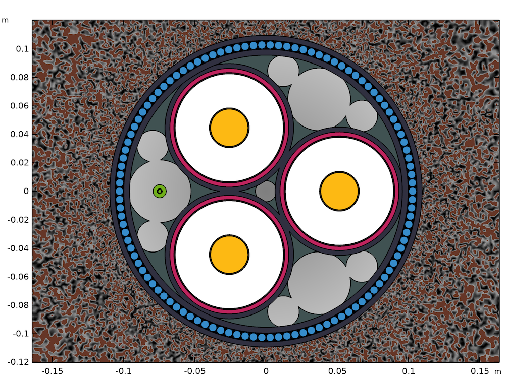
The beginning is a very good place to start, as most would say. Part 1 of the tutorial series is where you meet the model — a three-core lead-sheathed XLPE HVAC (cross-linked polyethylene, high-voltage alternating current) submarine cable with a twisted magnetic armor. You’ll also get a detailed overview on what to expect in the other seven parts of the series.
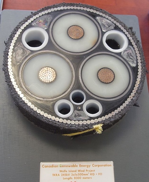
A submarine cable similar to the one modeled throughout this series. Image by Z22 — Own work. Licensed under CC BY-SA 3.0, via Wikimedia Commons.
This primer allows you to get acquainted with the user-friendly desktop environment of the COMSOL Multiphysics® software, and with numerical modeling in general. It shows you how to perform basic tasks, such as:
- Drawing or importing the 2D geometry
- Adding the material properties
- Creating selection filters
- Meshing your model
Feel free to skip ahead if you feel these topics are old hat to you.
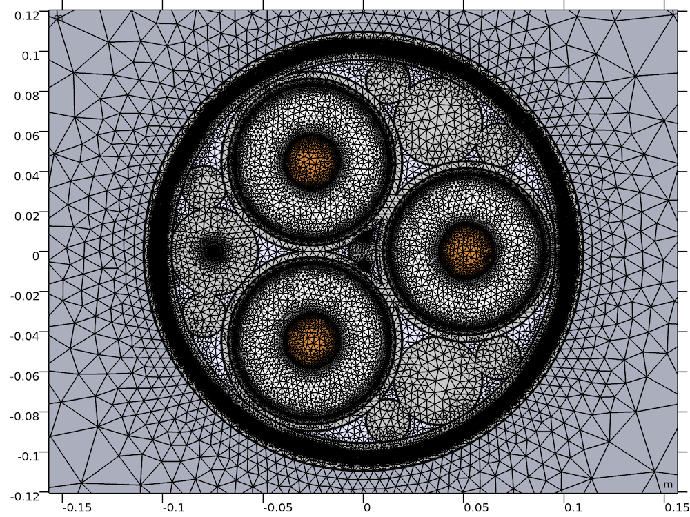
The cross section (left) and mesh (right) for a model of a typical lead-sheathed XLPE HVAC submarine cable with three cores. The geometry has been parameterized to allow for quick modification; any cable with the same basic structure can be investigated with ease.
Part 2: Capacitive Effects
The second tutorial focuses on modeling the cable’s capacitive properties and validates an important assumption: An analytical approach is sufficient for the analysis of the capacitance and charging effects. This will be useful throughout the series.
This tutorial is included for beginners, but the results also support the other parts of the series. It demonstrates the significance of the material properties and cable length. In the cross section of the cable model, the large contrast in material properties enables you to consider the XLPE as a perfect insulator and the lead and copper materials as perfect conductors. These results correspond to the analytical approximations.
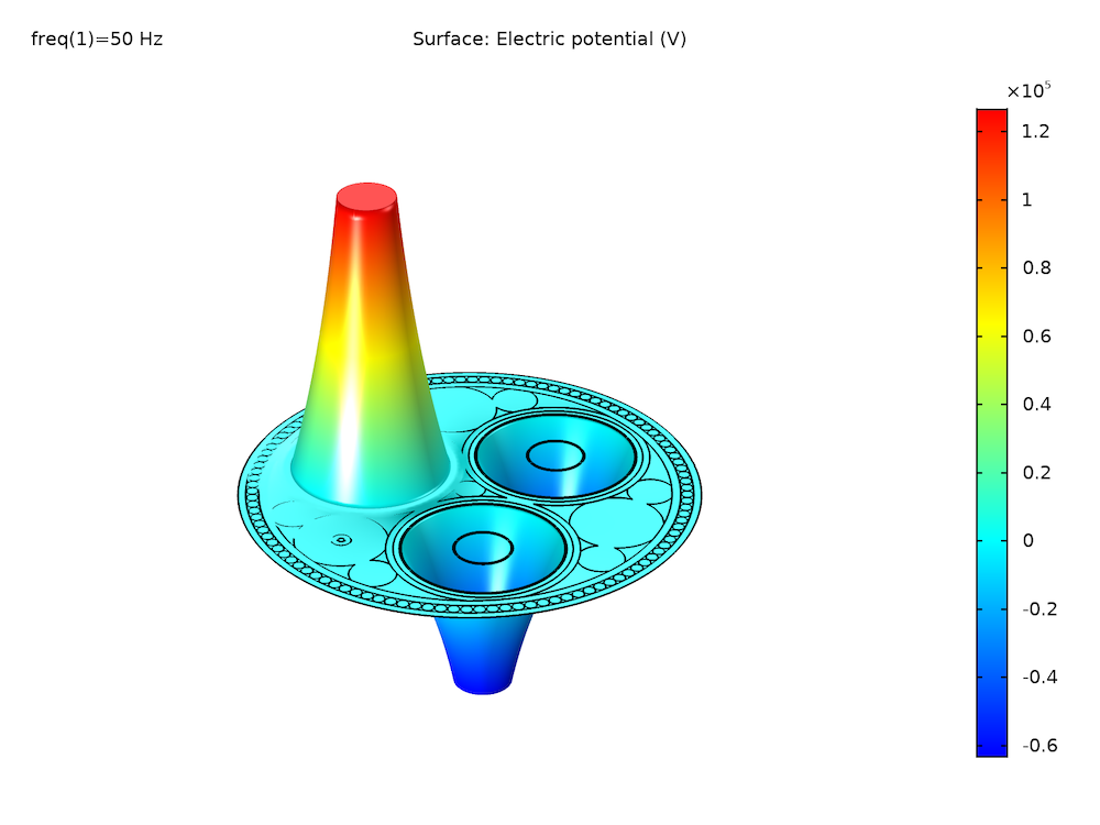
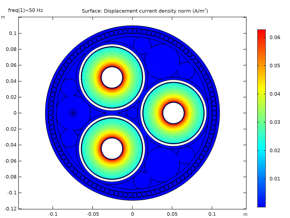
Left: The electric potential distribution after 10 km of cable for single-point bonding (at phase φ = 0). Right: The in-plane displacement current density norm in the insulators (primarily the XLPE).
In terms of cable length, you will see that the analytical approximations are sufficient for a 10-km cable. This stays true even under the worst possible nominal conditions, which occur when single-point bonding is applied and all voltage-inducing effects are in-phase.
Part 3: Bonding Capacitive
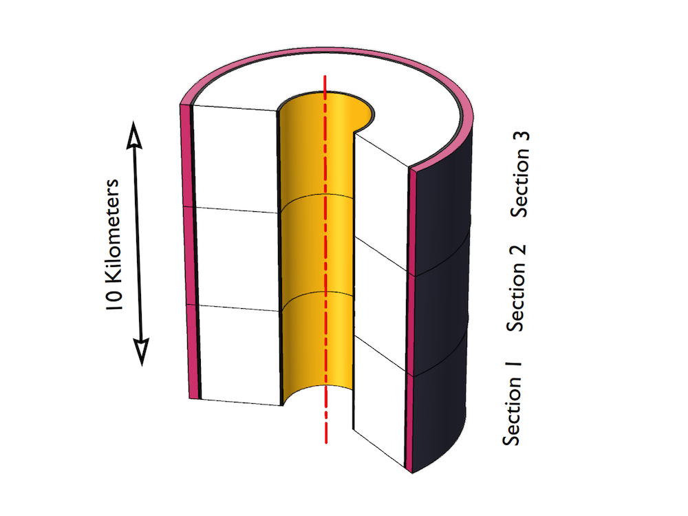
Part 3 of the series builds on the previous tutorial, which shows that you may neglect the capacitive coupling between the phases and consider one isolated phase. This reduces the model to an axisymmetric problem. In order to cover the full 10 kilometers of cable, we use a scaled 2D axisymmetric geometry in the model.
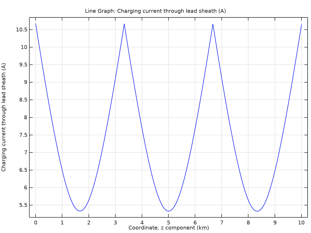
Left: The 2D axisymmetric geometry of an isolated phase with three separate bonding sections and a different scale for transverse and longitudinal directions. Right: The norm of the resulting charging current accumulated along the cable (for cross bonding).
The charging currents that leak into the screen build up along the cable and reach a maximum at the ground point, or intersection. The Bonding Capacitive tutorial analyzes the current buildup for different bonding types as well as the corresponding losses. The results are as follows:
| Bonding Type | Total Accumulated Charging Current at Ground Point/Intersection | Corresponding Losses per Screen |
|---|---|---|
| Single-Point Bonding | 55 A | 1.5 kW |
| Solid Bonding | 28 A | 0.38 kW |
| Cross Bonding | 10.7 A | 85 W |
Part 4: Inductive Effects
This part of the series builds on the previous two tutorials, which show that there is a weak coupling between the inductive and capacitive parts of the cable. In addition to this, 3D twist models will show you that although the field and loss distribution is a bit different in 3D, the lumped quantities (the resistance and inductance) computed by 2D and 2.5D models are actually quite accurate. To investigate this further, the Inductive Effects tutorial builds a 2D/2.5D inductive model that includes out-of-plane currents only.
Animation of the instantaneous magnetic flux density norm in the cable’s cross section, for solid bonding and with armor twisting included.
Animation of the current density induced in the cable’s armor and screens, for solid bonding and with armor twisting included.
The tutorial focuses on methods that allow you to approximate the wire twist in 2D, both for the magnetic armor and for the phases. For several configurations, the losses are evaluated. The configuration that has the armor twist included is referred to as a “2.5D model”, since it is a 2D model, with some 3D effects included. The twist suppresses the armor currents; the armor losses go down significantly, and the inductance goes up.
In addition to this, we demonstrate two different ways of modeling the central conductors. The first example assumes the central conductors to consist of solid copper, resulting in a typical skin- and proximity effect. The other shows a perfectly stranded Litz wire approach (a perfect Milliken conductor), resulting in a homogenized current density distribution. The simulation results found in this tutorial are validated using actual product data sheets following the official international standards. The comparison shows a good match, especially for the inductance.
Part 5: Bonding Inductive
The objective of Part 5 is to further examine the different bonding types that were introduced in Part 3 (and 4): single-point bonding, solid bonding, and cross bonding. (Cross bonding is especially of interest for terrestrial cable systems.) As opposed to Part 3, this part focuses on inductive effects.
You will learn how to individually consider three different cable sections by coupling three separate Magnetic Fields physics interfaces to a circuit. The resulting model allows for investigating debalanced cables and cables with dissimilar section lengths.
Furthermore, the tutorial demonstrates the effects of using a simplified geometry. Simplification is an overarching theme in this tutorial series: It is often justified to use a much simpler geometry than you think. You will see that it is not the amount of detail that makes a good model; it is the kind of details.
Part 6: Thermal Effects
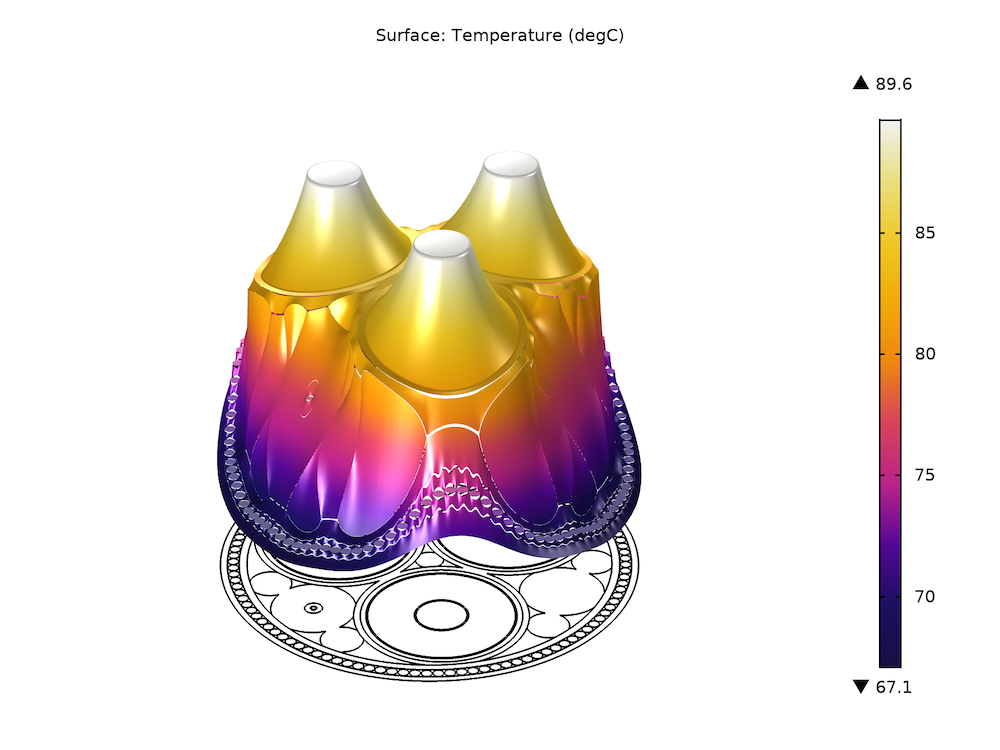
In Part 6, electromagnetic heating and temperature-dependent conductivity are added to the cable model. Building on Part 4, you’ll learn how to set up a two-way coupling between the electromagnetic field and heat transfer part by implementing a frequency-stationary study.
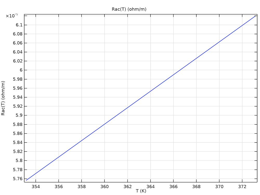
Left: An example of a preset resistance curve Rac (T). Right: The resulting temperature distribution when using a temperature-dependent conductivity such that Rac (T) is matched.
Results show the effect of temperature on losses for the cable’s phases and screens. When electromagnetic heating is added (without temperature-dependent conductivity) the cable heats up, but the electromagnetic properties are still identical to those reported in Part 4. When adding linearized resistivity to the phases specifically, the phase losses increase but not the screen and armor losses. The temperature reaches a maximum. If linearized resistivity is applied to the screens and armor as well, the temperature lowers and the losses decrease for both the phases, the screens, and the armor.
In this case still, the material properties are provided and the numerical model determines the corresponding AC resistance. However, for thermal cable models, it is common practice to use the temperature-dependent AC resistance as an input (as provided by the IEC 60287 series of standards, or as provided by a measurement). The final part of the tutorial demonstrates how to use any temperature-dependent resistance curve as an input and let the model determine the corresponding phase material properties. This is especially useful when you have a sophisticated Milliken conductor, and you are unsure what effective material properties to use (that is; without resolving the actual strands).
The results from these 2D models can be compared to those from 3D twist models. The 3D twist models are discussed in another blog post: Using 3D Models to Investigate Inductive Effects in a Submarine Cable.
Next Steps
Check out the Cable Tutorial Series if you’re looking for a self-paced electromagnetics modeling resource, whether you want to examine each section in detail or skip ahead depending on what interests you.
You can access the materials, which include step-by-step PDF instructions and MPH file downloads, via the button below:
You can also learn more about modeling cable systems by watching this archived webinar.




Comments (5)
Mohammad Ahli
February 15, 2018Hi,
Great study, Love the animations!
I just started reading about COMSOL, I haven’t used it yet, I need to learn the basics first. I cant wait to try the two ways of modelling the central conductor (solid and stranded litz). Just a couple of question, when does the approximation of perfect conductor and perfect insulator stop being accurate and to what percentage is it accurate roughly at the length of 10 km?
Thank you.
Durk de Vries
February 16, 2018 COMSOL EmployeeHi Mohammad,
>”when does the approximation of perfect conductor and perfect insulator stop being accurate and to what percentage is it accurate roughly at the length of 10 km?”
I assume you are referring to the approach discussed in part 2 of the tutorial. Here, analytical expressions are used to predict the cable’s capacitive properties. Numerical models and specification charts are used to investigate why, and to what extend these analytical expressions are valid.
The main equation of interest is for the cable’s capacitance C (typically given in [μF/km]). It assumes the cable’s phases (together with their screens) to be straight coaxial lines with a perfect insulator sandwiched between a perfectly conducting central core and a perfectly conducting screen:
C = 2πε/ln(R2/R1)
Apart from the cable’s non-perfect insulative / conductive properties, this approximation neglects the capacitive coupling between the three screens, and the capacitive coupling between the screens and the soil. The main question is whether this approximation holds, even when using single point bonding for a 10[km] long cable, embedded in wet soil.
Numerical modeling tools are ideal for investigating this, as you can easily test different scenarios without having to actually install 10[km] of cable. Even when considering the fact that a numerical model itself is an approximation of real world conditions, you can extract some pretty important knowledge.
For example: as opposed to many other material properties (such as permittivity ε, or permeability μ) the conductivity σ is able to cover an incredibly large range. It can be as small as 1e-18[S/m], or as large as 6e7[S/m]. Even when adding all kinds of parasitic effects (while still avoiding electromagnetic breakdown), it turns out the XLPE is such a good insulator that it completely dominates the capacitive part of the electromagnetic problem.
If you want a figure: for this particular cable design working under nominal conditions, the capacitance and charging current deviates from the “ideal” value by about 0.5-1% or so. If the phases and screens are twisted around the cable’s center, their effective length will be a bit longer, adding a bit more to the total current leakage.
More important than the figure itself perhaps, is the observation that these effects are rather small, compared to the effect when changing the XLPE’s material properties a bit, or its radius / “roundness” (as predicted by the analytical model). These (“ε”, “R2/R1″) are therefore very important design parameters.
>”I haven’t used it yet, I need to learn the basics first.”
The Cable Tutorial Series is written with this in mind. If you need further support, feel free to contact our sales department.
ali Hosseini
March 29, 2019Hi,
I am trying to simulate a 3 phase single core conductor with a metal sheath.
But the graf of the induced voltages in the sheath are not the same as the analytical method.
The second section of cross bonding should be a parabola down wards and not up.
is the analytical method wrong or the simulations?
Brianne Christopher
March 29, 2019 COMSOL EmployeeHello Ali,
Thank you for your comment.
For questions related to your modeling, please contact our Support team.
Online Support Center: https://www.comsol.com/support
Email: support@comsol.com
Faouzi Hassaine
March 23, 2022Modeling Cables in COMSOL Multiphysics®: 8-Part Tutorial Series :
In the alternating current, the voltages are of the same effective value out of phase with respect to each other, by an angle of 120°
but in this tutorial the voltage between the three phases are not of the same amplitude, why doesn’t the same?