Multiparameter Optimization with a Least-Squares Objective

Optimization is an efficient way to gain deeper knowledge of a model. Much like the different flowers in a colorful bouquet, you can perform a variety of different optimization projects using the Optimization Module. However, parameter estimation is also a widely used technique. Such an analysis is usually set as a least-squares problem based on measured data, but for a clear and unique answer, you might need multiple measurements. Today, learn how to estimate parameters using a multiparameter data set.

Using Multiple Data Sets

When performing laboratory experiments, you rely on the precision and accuracy of the — often used — measurement equipment. While plenty of information is available in the equipment specifications, it usually applies to new, well-calibrated systems. However, you might forget to calibrate your devices, or the system shows a systematic bias due to wear and other processes.

If you have a data set exhibiting such errors, it is important to correct them so that you can analyze the measured data accurately. An applied example is an experiment of flow through a column, where you inject a chemical and record the breakthrough curve at the outlet. For further analysis, the set flow rate of the pump is used. However, due to calcification, the flow rates are systematically biased. Performing a multiparameter optimization with various flow rates enables you to obtain a factor to correct all of the data.

Multiparameter Optimization of a Transport Problem

This optimization problem is based on a transient model using the COMSOL Multiphysics® software and Transport of Diluted Species interface. A complete model is a prerequisite for the optimization step. The model discussed here is set in 1D and has a geometry with a column that is 1 m in length.

For the transport properties, you can set the flow velocity, which is simply the flow rate multiplied by the opening width of the column. Further, you can assign Inflow and Outflow boundary conditions and a Dirichlet boundary condition at the inlet, set to a fixed concentration.

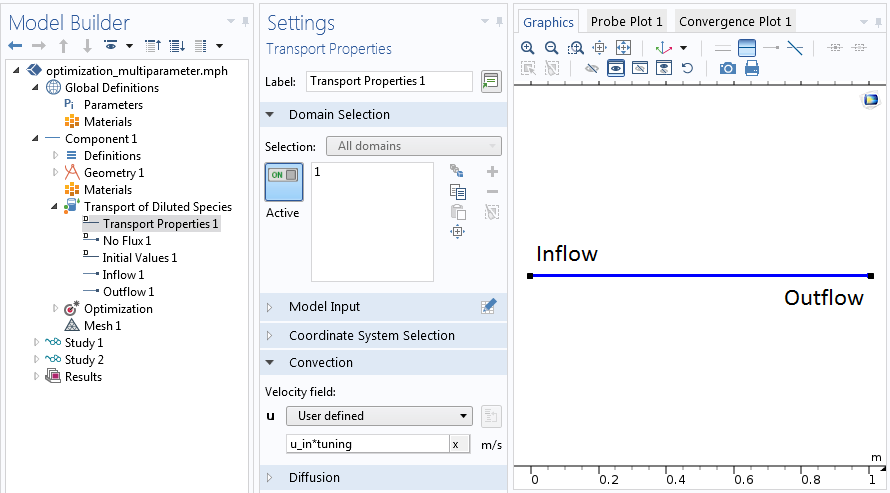
Setting up the physical problem prior to the optimization.

While the true velocity of the problem is unknown, you can rewrite it as the product u_in*tuning. Here, u_in represents the set flow rate and tuning of the global correction factor, which derives directly from u_in=Q/(A*tuning). Hence, tuning accounts for the area change of the system.

In optimization jargon, u_in is the experimental parameter identifying the individual experimental runs. The obtained concentration is our least-squares objective, which is compared to measured data, and tuning is the control variable.

Setting Up the Optimization

Starting with the complete physical model, you can add two items to transform it into an optimization model. First, the Optimization interface in our example has two nodes: Objective and Control Variable. For any optimization study, these nodes are a prerequisite.

While there are many feasible optimization objectives, the least-squares objective is well defined and from the shape Sum_i(u_obs_i-u_sim_i) 2. Hence, it minimizes the sum of the distances between all given data points.

Due to the strict formal approach, there is no need to express the objective function. However, you need a data file that contains all information needed for a least-squares objective. It is important to note that the data file needs to be structured in columns. You can assign the individual columns in the subnodes.

Note that the order of nodes in the Model Builder tree (from top to bottom) corresponds to the order of columns in the data file (from left to right). It is also important that every column of the data file is identified by an appropriate subnode.

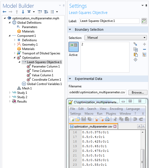
Assign the nodes in the least-squares objective (top down) to the semicolon-separated columns (left to right) in the data file.

The transport optimization example requires four columns:

Parameter Column

In the example, you set the identifier u_in in the parameter column. This is the flow rate of the pump used to discriminate between the different experiments as well as the same parameter that is assigned under Global Definitions > Parameters. You can also find this parameter used for the transport properties in the Transport of Diluted Species interface.

Time Column

The times stated in the data file need to be in SI units, seconds. However, in general, these times don’t need to match the stored output times accurately. Nevertheless, good accuracy is still recommended.

Value Column

In the value column, you give the expression, which is evaluated from the numerical model outcome. This should be entered in the way that it represents the exact metric of the recorded data. Variable Name refers to the measured data, which can be accessed during postprocessing by using such a name.

Coordinate Column

The stated coordinate in the file is the destination where measurements are made. There is also one specialty that must be considered: The number of coordinate columns in the data file must be the same as the dimension of the geometry, even when the selected Least-Squares Objective feature is on a lower dimension. In that case, model expressions are evaluated at the nearest points on the given selection.

Adding the Optimization Study Node

Here, you make two adjustments by setting the method to the well-known Levenberg-Marquardt algorithm, designed to tackle least-square problems efficiently. Since the goal is to perform a multiparameter study, you can switch the least-squares time/parameter method to: From least squares objective. The other settings can be left as default for now.

The correct time-stepping and parameter sweeps are recognized directly from the data file and there is no need to set it individually in the Step 1: Time dependent settings. Eventually, using such settings, the solver can sum up all squared deviations for all time steps and parameters, as well as search and minimize such sums by finding a global correction factor that is appropriate for all individual experiments.

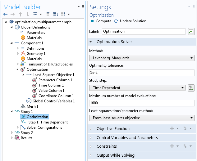
Settings of the Optimization study step.

Conclusion

With all of these settings, you have a very generic model that can be applied to many experimental runs by updating only the underlying data file. The settings automatically adjust the model to the experimental parameters. So far, this includes variations of the amount of experimental parameters’ recorded sample times.

Such models could be easily extended to consider more parameter variations; e.g., variations of input concentration or more measurement locations in an analog manner. Further steps could be used to transform a model into an application, where you can freely choose the length of the column, hence the geometry. This way, you end up with a powerful tool to evaluate your experiments and assure their quality.

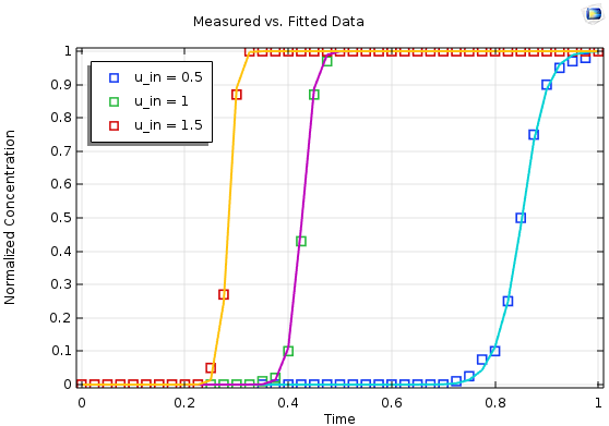
Results for a multiparameter fit based on three individual measurements (symbols) with the simulated and optimized output (lines).

Further Resources

• Try a liquid chromatography tutorial model:
  • Liquid Chromatography
• Read this related blog post:
  • Fitting Measured Data to Different Hyperelastic Material Models