
Last month, my colleague Ruud described some of the most effective ways to use arrow plots in your COMSOL Multiphysics simulation results. In this next installment of the postprocessing series, I’ll continue with slice plots, which are an easy way to visualize physics behavior on many different parts of your model.
Using Slice Plots to Visualize Fluid Flow Across a Pipe
Slice plots, which can be applied to many model types, show a cross-sectional surface (sometimes several of them) that indicate how a variable changes over a distance or a specific area of the plot.
If you recall Ruud’s last post, he demonstrated arrow plots by using the Flow in a Pipe Elbow model. Let’s continue with his example and investigate slice plots as another tool to help us understand the velocity and pressure drop across the pipe.
The two figures below, which might ring a bell if you read Ruud’s last post, show slice plots that travel through the entire pipe:
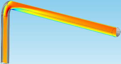
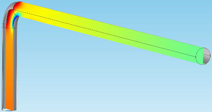
These visuals give a very clear, immediate picture of what’s happening to the flow in the center of the pipe. This is done by plotting a virtual surface that vertically slices the geometry down the middle.
Creating the Slice Plots in COMSOL Multiphysics
To create these slice plots, we can add a new 3D plot group in the Flow in a Pipe Elbow model. Following that, we can head up to the ribbon and choose Slice from the 3D Plot Group tab.
Note: In the version I present here, I have added some plot outlines and a gray surface to help give a feel for the pipe shape — to give it a wall, if you like. I’ve also mirrored the main solution so that a centered slice plot will bisect the entire pipe geometry and not the half that was originally modeled. This makes for better visualization for the purpose of this blog post.

When you click the Slice feature in the ribbon, you’ll probably notice that the software plots a series of planar surfaces within the pipe, by default.
Let’s take a look at the settings:
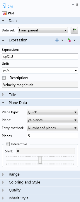
COMSOL Multiphysics automatically plotted the velocity on five surfaces that lie on yz-planes and shift in the x-direction. If we change the Plane field to xy-planes and the number of planes to 1, we’ll see Ruud’s original slice plot, which is shown above.
Now, let’s take a closer look.
If we return to the default plot, with five yz-planar surfaces, we’ll see this:
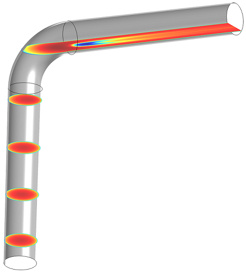
Here, it’s very easy to see the velocity inside the pipe.
There’s also a simple way to move the slices around, so that we can see the velocity in different areas. If we select the Interactive checkbox, we can use the slider to shift the surfaces in whichever direction the planes don’t depend on. In this case, we’ll shift the surfaces in the x-direction:
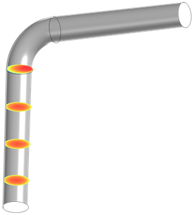
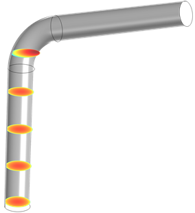
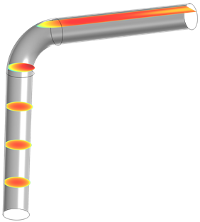
As we can see, this will become especially useful for when you want to create an array of multiple slice plots, but don’t want them to interfere with each other.
Defining the Right Plane
Suppose that we want to see the velocity on a slice right in the pipe bend that is perpendicular to the wall. Let’s change the plane type to General and choose Point and normal for the entry method. This will allow us to create a diagonal plane in the right-angle bend. However, it’s important to make sure that the plane is correctly oriented.
In order to choose the right point and vector, let’s first take a look at the parameters. These can be found under the Global Definitions node:
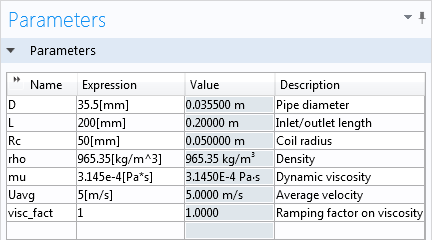
The inlet and outlet length, or the length from one open end of the pipe to the bend, are represented by the variable L. This accounts for most of the vertical distance that we’ll want to apply to our plane. The variable Rc gives the radius of the bend, so let’s also add that to the distance, making the x-coordinate L+Rc.
The normal vector needs to be tangent to the direction of flow around the bend, so in the direction of (1,1,0) at the location of the point.
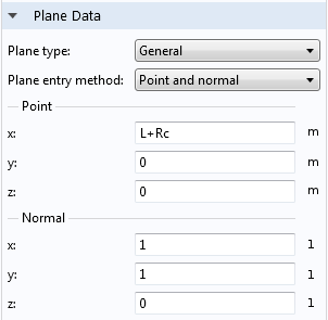
Here’s what it looks like:
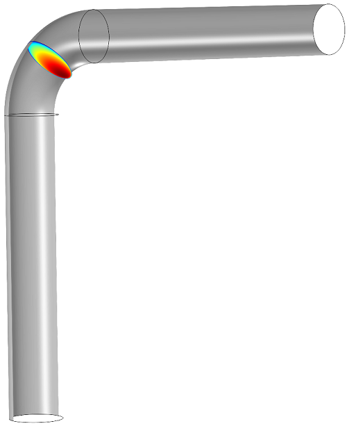
This diagonal slice shows the velocity gradient as the fluid changes direction to follow the pipe. The fluid is moving slowest on the outside of the curve and faster toward the inside.
Now we can add a few slices, defined by yz-planes and xz-planes, to tell us the velocity in the horizontal and vertical sections of the pipe.
Tip: I did this by duplicating the original slice plot twice, rather than creating two new plots. I also chose Slice 1 under the Inherit Style tab in the settings for both of the duplicate plots, so that the color and data ranges will be the same for all three.
The locations of the points that will define these slices are (L,0,0) and (L+2*Rc,Rc,0), which will place planes on either side of the bend, where the curve begins and ends. Their respective normal vectors are (1,0,0), and (0,1,0):
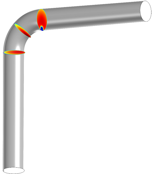
What happens if we check the Additional parallel planes box? In the Slice 3 plot, it will create a series of surfaces that run parallel to the one created by the plane data:
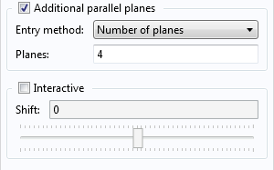
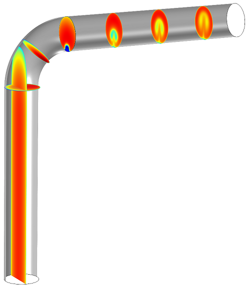
This looks a little messy, but bear with me for a minute. Remember that interactive slider we saw earlier? If we want to get rid of that long surface in the vertical section of the pipe, we can shift everything over a little. If all the surfaces are shifted by 0.035, the planes don’t overlap:
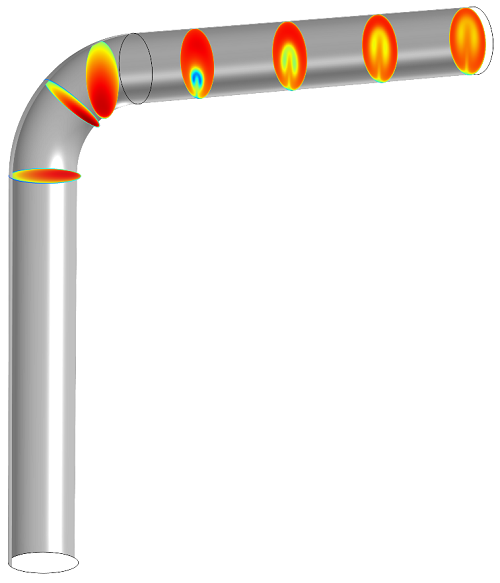
We can repeat this process with the horizontal surfaces (whose normal vector is (1,0,0)):
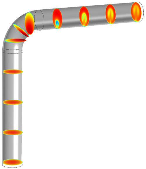
Now the series of slice plots shows the velocity change in a cross section as water flows through the pipe, with the fluid flow becoming more turbulent after the bend.
That’s it for a brief introduction to slice plots. Stay tuned for our next installment in the postprocessing series: contour and isosurface plots.


Comments (5)
Malkhaz Meladze
December 2, 2014So simple … if you know how! It was easy to follow and repeat.
Thank you!
Reed Teyber
January 19, 2017Thanks! but what if you want another plot type in the plane, i.e. instead of a magnitude surface, show streamlines in the plane?
Ruud Borger, COMSOL employee
January 20, 2017Hi Reed,
That’s an interesting question. For streamlines in a plane, you need to use a different method. First, in “Data sets”, you need to create a “Cut plane”. Then, you can create a 2D plot which uses said Cut plane, in which you can add streamlines, or other types. A more extensive guide on how to do this can be found on page 16 of our “Essentials of Postprocessing and Visualization” manual. You can find this via File => Help => Documentation.
(Note: If you only want to plot arrows in one plane, then you can combine that with Lexi’s instructions.)
I hope that clears things up, please let me know if you have additional questions.
Juan Gomba
May 2, 2017Hi Ruud, Reed,
I am interested in exactly that option,ç: show the streamlines that cross a surface. We would like to plot a set of streamlines, of given starting points in the entrance of a pipe, emerging a cross section at the outlet.
We can see the inlet but at the outlet the plot has no sense. Could you please give us a detailed way to achieve this graph?
Caty Fairclough
May 8, 2017Hi Juan,
Thanks for your comment!
For questions related to your modeling, please contact our Support team.
Online Support Center: https://www.comsol.com/support
Email: support@comsol.com