Why Should I Use Automatic Wall Treatment for My CFD Modeling?

Wall-bounded turbulent flows display extreme gradient close to the walls. The most accurate way to treat these gradients is to resolve them using a low Reynolds number model, which is computationally expensive. Industrial applications use wall functions, which model the flow closest to the wall rather than resolving it. Wall functions are robust and efficient, but not particularly accurate. New automatic wall treatment functionality in the COMSOL® software combines the benefits of wall functions and the low Reynolds number model.

How Automatic Wall Treatment Works

The new automatic wall treatment functionality in COMSOL Multiphysics version 5.3 combines the robustness of wall functions with the accuracy of low Reynolds number models by adapting the formulation to the mesh available in the model. If the boundary layer mesh is coarse, a robust wall function formulation is used. If the boundary layer mesh is dense, a low Reynolds number formulation is used, which resolves the velocity profile all the way to the wall.

The transition between the low Reynolds number formulation and the wall function formulation is smooth and is done by blending the two formulations in the boundary elements. By calculating the wall distance of the boundary elements’ grid points in viscous units given by a liftoff, the combination of the two formulations is used for the boundary conditions.

The figure below exemplifies the transition between the low Reynolds number formulation and the logarithmic wall functions for the low Re k-ε turbulence model. The wall distance in viscous units, y+, is plotted against the turbulence dissipation rate, ε. The green curve represents the low Re formulation of ε, the blue curve is the wall function representation, while the red curve is the Wolfshtein model that is used for the automatic wall treatment. Observe the smooth transition obtained with the Wolfshtein model (red) for y+ values ranging from 1 to 20; i.e., in the buffer layer.

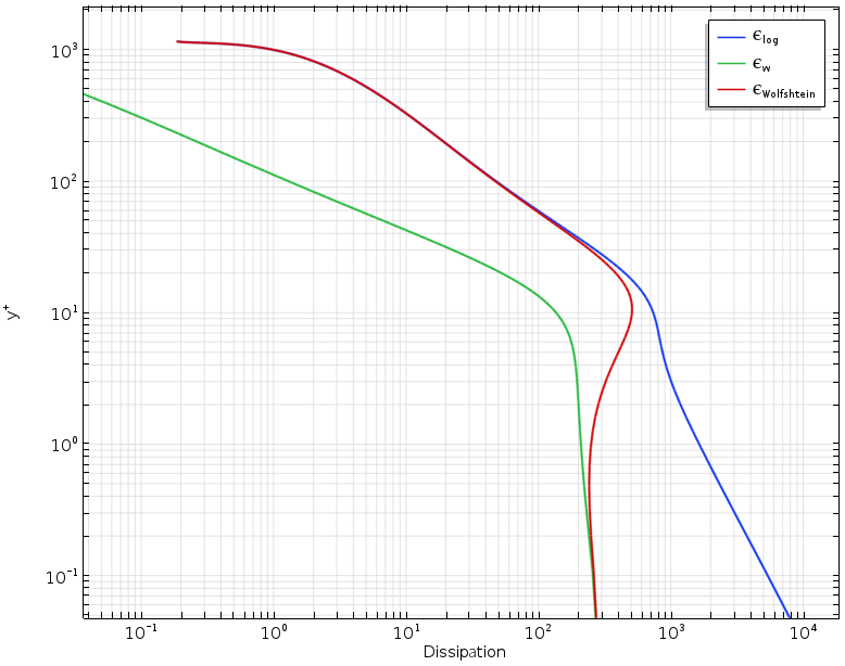
Low Re formulation (green), wall functions (blue), and automatic wall treatment (red).

In order to verify the definition of a model, we can investigate how the walls are treated by plotting the y+ variable at the boundaries, as shown in the figure below. For this pipe elbow benchmark model, we can see that the low Reynolds number formulation dominates at the inner curved surface of the bend, while at the straight sections of the pipe, the wall function formulation dominates.

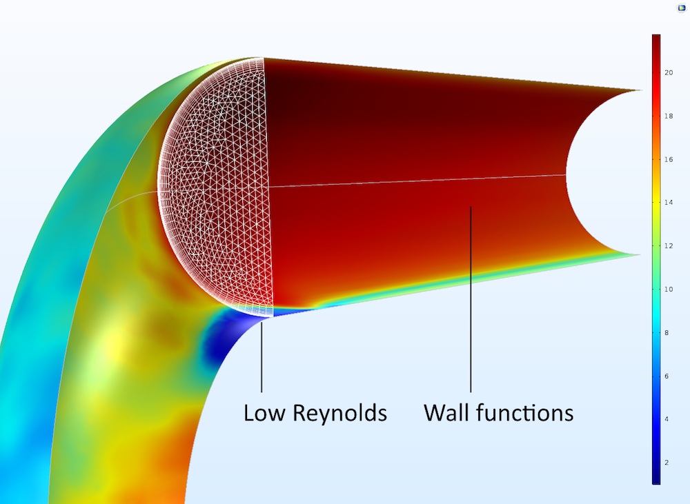
The deep red regions have a value of y+, or around 20, while the blue regions are at around 1.

Addressing a Wide Range of Problems with Automatic Wall Treatment

The functionality for automatic wall treatment allows the use of low Reynolds number models for a wider range of problems. Examples are coupled problems where certain surfaces are subjected to flux of heat, chemical reactions, or fluid-structure interactions. Instead of having to use a dense mesh on all surfaces, which could be very computationally expensive, we can apply a dense mesh only on the relevant surfaces where we need to accurately resolve the boundary layer.

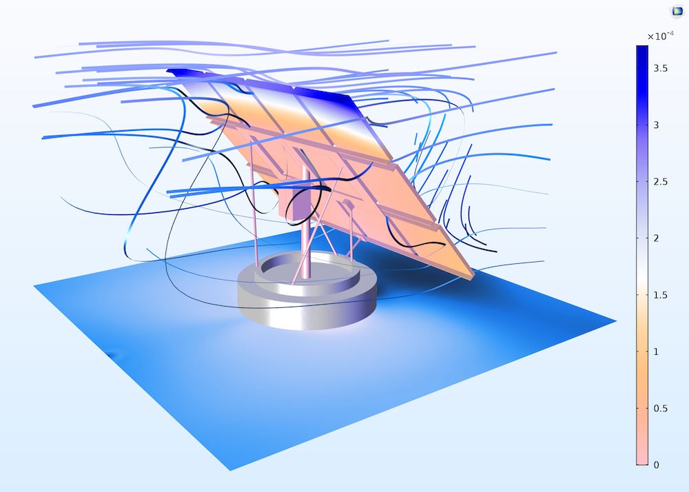
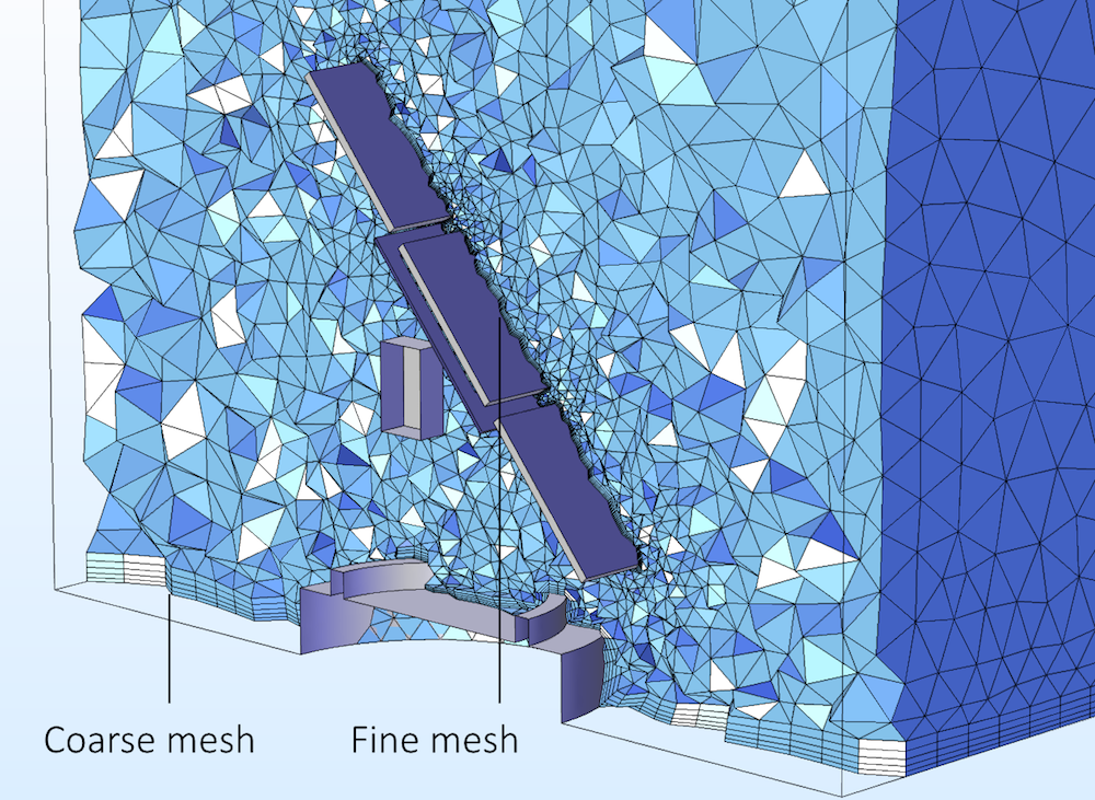
The figure below shows the boundary layer mesh for the solar panel model in the Application Library. We can see that the mesh on the surface of the panels is dense with tight boundary elements. On these surfaces, we need the forces exerted by the fluid on the structure with high accuracy in order to compute the stresses and strains as well as the displacements. The concrete base is not influenced by the forces of the wind and the forces on these surfaces do not require the same accuracy. The automatic wall treatment functionality allows for the solution of this problem by just clicking the Compute button, while a conventional low Reynolds number model would require a dense boundary layer mesh on all boundaries in order to converge.

In this fluid-structure interaction tutorial of a solar panel, we can use a coarse boundary layer mesh for the ground and the concrete foundation and a fine mesh on the surface of the panels, where the forces need to be calculated with accuracy.

Simplified Model Development

The new functionality is also of great use in model development. In order to iron out the proper assumptions and boundary conditions, we may need quick results on a coarse mesh as a first step. Once we have verified our model formulation, we can refine the mesh in order to obtain more accurate results. The automatic wall treatment functionality allows for this type of model development with a minimum number of obstacles and operations: the “only” thing we need to do is to refine the mesh.

The robustness that this new functionality provides also simplifies the use of low Reynolds number turbulence models in general. A common procedure is to solve the model equations using wall functions with high Reynolds number models and then use this solution as the starting guess in the low Reynolds number models. The adaptive wall treatment reduces this procedure to the sequential solution of the model equations for a coarse and fine mesh; i.e., it eliminates the need for the formulation and solution of a high Reynolds number model as a first step.

Turbulent Flow Interfaces

Automatic wall treatment is available for all low Reynolds number turbulence model interfaces in the latest version of the CFD Module:

• k-ω
• Low Reynolds k-ε
• SST
• v2-f
• Spalart-Allmaras
• L-VEL
• Algebraic y+

The automatic wall treatment functionality is available in the Settings windows for all of the above-mentioned flow interfaces. The figure below shows the selection for the Turbulent Flow, k-ω interface. In this flow interface, we can select from three different wall treatment options: automatic, wall functions, and low Reynolds number.

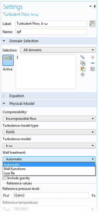
The three available options for the Turbulent Flow, k-ω interface: automatic, wall functions, and low Reynolds number.

Further Resources

• Try these example models yourself to see the automatic wall treatment functionality in action:
  • Flow Through a Pipe Elbow
  • Airflow over an Ahmed Body