

Acoustic traps offer a contact-free method of manipulating cells and particles for a wide range of biomedical applications. In a typical acoustic trap, a piezoelectric transducer induces a pressure field in a fluid, generating acoustic radiation forces that effectively trap small objects suspended in the fluid. In this blog post, we will take a closer look at a model of an acoustic trap — with thermoacoustic streaming and particle tracing included.
A Brief Introduction to Acoustic Trapping
August Kundt first demonstrated that sound waves can exert acoustic radiation forces on exposed particles in 1874. Since the 1990s, this principle has been utilized in microfluidic devices and lab-on-a-chip systems, and, today, commercially available acoustic traps are used in life science laboratories and medical facilities around the world. Acoustic trapping systems have a variety of applications, ranging from the enrichment and purification of low-concentration samples to studies of cell–cell interactions, particle sorting, and the isolation of bacteria, viruses, or biomarkers for point-of-care diagnostics.
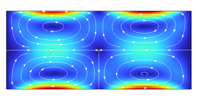
Figure 1. Acoustic streaming flow in a cross section of a microfluidic channel, which can, for example, be used for upconcentrating or separating particles in biological fluid samples.
The acoustic waves induced in acoustic traps give rise to acoustic streaming, or rapidly moving vortices around the trapping site. The acoustic streaming results in a viscous drag force on the particles in the fluid. The particles are also subject to an acoustic radiation force. For large particles, the acoustic radiation force is dominant, while for small particles, the drag force is dominant. The particle size at which the dominant force changes depends on the specific device and the acoustic properties of the particle. In most devices, the acoustic radiation force is used to trap or control particles; therefore, the drag force from the acoustic streaming field will typically prevent small particles below a critical size from being captured by the acoustic trap.
With this information in mind, let’s dive into how an acoustic trap can be simulated in COMSOL Multiphysics®. The 3D Acoustic Trap and Thermoacoustic Streaming in a Glass Capillary model discussed in this blog post is available for download from the Application Gallery.
Modeling an Acoustic Trap
The 3D model geometry for our acoustic trap is shown below. The trapping system’s geometry is divided along its two symmetry planes, allowing us to model just one quarter of the system. A quarter of a small piezoelectric transducer (gray) is placed under a quarter of a glass capillary (yellow) filled with water (blue). Since in actuality the ~5-cm glass capillary is very long compared to its height of 0.48 mm and width of 2.28 mm, its ends are modeled using a perfectly matched layer (PML). A PML is a domain that can be added to a geometry to simulate the attenuation and absorption of all outgoing waves. The PML comprising half of one end of the capillary is shown in green below. As you can see, the PML is active in the glass capillary as well as in the fluid in this model.
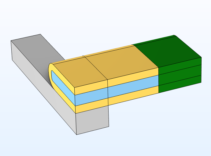
Figure 2. Model geometry of one quarter of the acoustic trap.
Modeling an acoustic trap is a true multiphysics problem involving electromagnetics, solid mechanics, acoustics, fluid flow, and, in some cases, heat transfer. An oscillating voltage difference across the piezoelectric transducer induces vibrations in the piezoelectric material and thus also the glass capillary. This piezoelectric effect is modeled by coupling the electrostatics in the piezoelectric transducer domain with the solid mechanics of the piezoelectric transducer and glass capillary. To model the resulting pressure field in the fluid, a multiphysics acoustic–structure interface at the boundary between the glass capillary and the fluid is used to couple the solid mechanics with pressure acoustics.
Additionally, the dissipation of energy in the piezoelectric transducer heats up the system, resulting in a temperature gradient in the glass capillary and fluid that, in turn, generates gradients in the acoustic properties of the fluid that affect the acoustic streaming. A multiphysics coupling for nonisothermal flow takes the effects of this temperature gradient into account, combining modeling of the heat transfer of the entire geometry (solids and fluid) with a creeping flow model in the fluid domain. A coupling between the creeping flow and pressure acoustics is used to model the acoustic streaming. Finally, to see if our acoustic trap works as intended, particle tracing is used to determine the trajectories of two types of particles in the fluid, large silica glass particles and small polystyrene particles.
Let’s take a look at the results!
Simulation Results
Acoustic Fields
The acoustic fields are modeled in the frequency domain. The system is actuated in the ultrasound regime at a frequency of 3.84 MHz. The frequency corresponds to a standing half-wave resonance in the height of the fluid chamber. The electric field in the piezoelectric transducer, the displacement field in the piezoelectric transducer and glass capillary generated by the piezoelectric effect, and the resulting acoustic pressure field in the fluid are shown below. The acoustic field contains a minimum pressure region, called a pressure node, above the piezoelectric transducer.
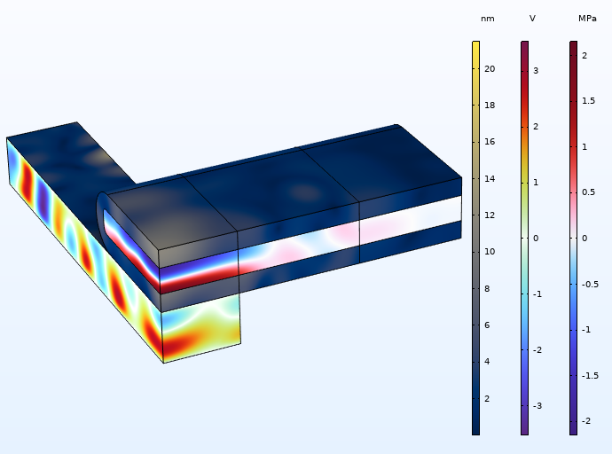
Figure 3. Displacement field (nm), electric field, and pressure field in the acoustic trap.
The acoustic radiation forces acting on a particle in an acoustic field can be described by the Gor’kov potential. Figure 3 shows the Gor’kov potential computed for the small polystyrene particles in our model. Particles suspended in the fluid will be pushed to the minimum Gor’kov potential and thus should be trapped in the center of the glass capillary. For a detailed discussion of the acoustic radiation force and how to compute it using COMSOL Multiphysics®, check out this previous blog post.
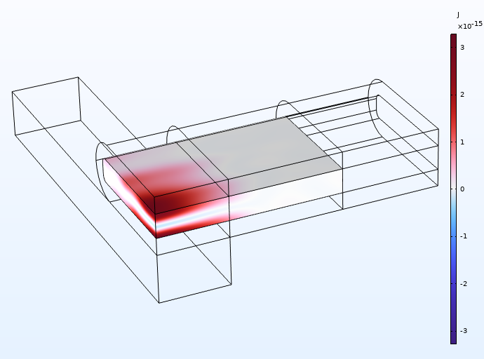
Figure 4. Gor’kov potential for polystyrene particles with a diameter of 1 µm.
Thermoacoustic Streaming
What about acoustic streaming? The simulation results below show four streaming rolls above the piezoelectric transducer, which can only be explained by the temperature field. The temperature gradient in the glass capillary and fluid induced by the heating in the piezoelectric transducer creates gradients in the fluid density and compressibility. These gradients in the fluid material parameters, together with the acoustics, lead to the thermoacoustic body force, which drives acoustic streaming and results in this characteristic streaming pattern.
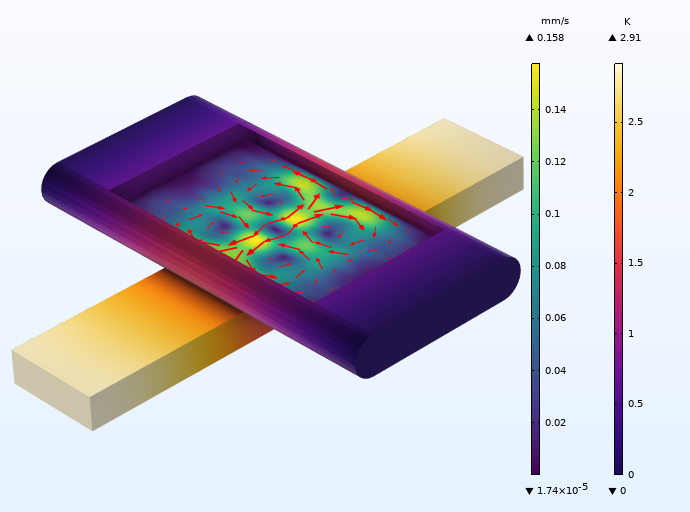
Figure 5. Thermoacoustic streaming inside the glass capillary and temperature gradient. The symmetry planes of the geometry are folded out.
Particle Trajectories
Using particle tracing, we can also find out whether particles with certain properties will be drawn into the acoustic trap. The following animations show the computed trajectories of large silica glass particles with a diameter of 10 µm and the trajectories of smaller polystyrene particles with a diameter of 1 µm. The silica glass particles above the piezoelectric transducer move towards the center of the glass capillary and are trapped there, while the movement of the smaller polystyrene particles is governed by the streaming flow.
Figure 6. Particle trajectories of large silica glass particles.
Figure 7. Particle trajectories of small polystyrene particles.
Try It Yourself
Interested in trying this multiphysics model for yourself? Click the button below to download the MPH file:
Further Reading
These additional tutorial models featuring acoustic streaming and acoustic traps are also available in the Application Gallery:


Comments (0)