Learning Center

Setting Up the Laminar Flow Interface

In this part of the course, we'll cover how to set up the Laminar Flow interface in COMSOL Multiphysics^® for a magnetohydrodynamics (MHD) model.

For a general introduction to modeling with the Laminar Flow interface, see "Basics of Modeling Laminar Flow in COMSOL Multiphysics". This article includes a video that offers a detailed demonstration of using the interface.

Defining Flow

Inlets

When an Inlet condition is added to a model, it allows boundaries where there is a net flow of fluid into the domain to be defined. The Inlet condition includes several methods for describing the distribution of the fluid velocity across the inlet: Velocity, Fully developed flow, Pressure, and Mass flow.

Each of these conditions represents different physical situations and has their own benefits and drawbacks to using them in an MHD model.

Velocity

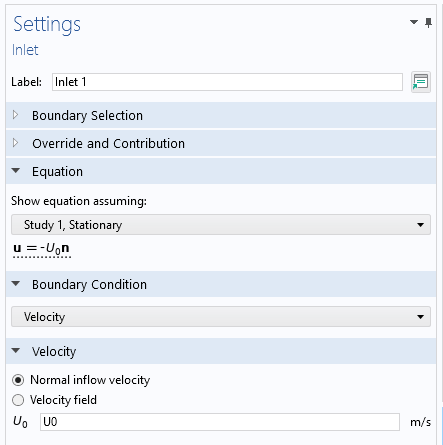
The settings for the Inlet feature using the Velocity option.

The Velocity option allows either the normal inflow velocity or the velocity field to be specified with an analytic expression.

If a developed MHD flow profile is needed on the inlet, such as the Hartmann flow profile, the Velocity option can only be used if the analytic expression for that flow profile is known. This situation is rare, but when it occurs, it allows this flow profile to be applied without having to solve for it by adding extra variables in the solver to calculate the profile, which saves computation time.

Alternatively, the Velocity option can be used in the case of a uniform flow profile to set the fluid velocity to a constant value across the inlet.

Pressure

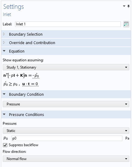
The settings for the Inlet feature using the Pressure option.

The Pressure option applies a fixed pressure across the inlet boundary and solves for the flow profile on the inlet.

This condition is capable of solving for the magnetohydrodynamic profile on the inlet, allowing a flow that has fully developed to be applied. This is particularly useful for simulating duct flow in a uniform background field, as it allows a relatively short section of the duct to be simulated while still representing an infinite duct. In addition, since many MHD models specify a driven fluid by giving a pressure drop or pressure gradient, this is most naturally applied by constraining the pressure on the inlet.

When working with high Hartmann numbers, certain combinations of wall conductivity lead to a reversed flow direction. This behavior can be included in the inlet flow profile when using the Pressure option by disabling the Suppress backflow option. The backflow suppression method works by varying the pressure on the inlet until no backflow occurs. This option should also be disabled if a constant inlet pressure is needed.

The drawback of using the Pressure option is that in order to calculate for the flow profile, an additional equation must be solved for on the inlet. This additional equation often increases the computation time.

Mass Flow Rate

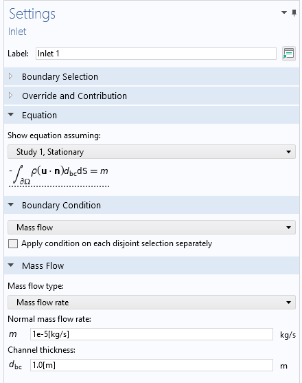
The settings for the Inlet condition using the Mass Flow option.

The Mass flow rate option allows the mass flow rate for the fluid to be specified, and then it solves for a constant pressure across the inlet and the corresponding flow profile to give the required integrated mass flow across the inlet.

When the fluid is incompressible, this condition essentially combines the pressure option with the ability to specify the average fluid velocity on the boundary rather than having to fix the pressure.

In this case, a value is entered in the Mass flow rate option, a pressure is set on the boundary, the flow profile is solved, and then the applied pressure is varied to match the mass flow rate. This process solves two equations: one for and one for on the inlet. Solving these equations can significantly increase the computation time for the model.

Fully Developed Flow

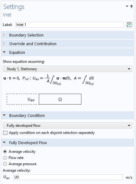
The settings for the Inlet feature using the Fully developed flow option.

The Fully developed flow option solves for a flow profile on the inlet, given an average velocity or pressure over the inlet, through the following steps:

Virtually extending the length of the inlet Solving for the flow profile by projecting the solution of the momentum equation in the virtual inlet onto the boundary
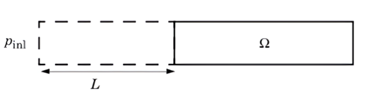
Identifying the flow profile on the inlet using the Fully developed flow option. The physical modeling domain is on the right, and the inlet on its left boundary is virtually extended backward by a distance of . A pressure of is applied across the new virtual inlet.

This method attempts to account for the effect of any volume forces; however, in MHD models, it tends to underrepresent the dampening effect of the Lorentz force. The generated flow profile then sits somewhere between the laminar flow profile and the true magnetohydrodynamic profile. The underrepresentation can be resolved in certain cases by including an additional lead-in section of pipe between the inlet and the region of interest where the flow can develop fully into the magnetohydrodynamic profile.

The charts below show how the flow profile is formed for a Hartmann number of 10 and 100. To show this development, the changing flow profile is plotted at a series of distances D from the inlet, where D is defined in terms of the plate half-separation d. At a Hartmann number of 10, it takes a distance of around 7.5d from the inlet for the flow to form the Hartmann flow profile, while at a Hartmann number of 100, only a distance of 2d is required.

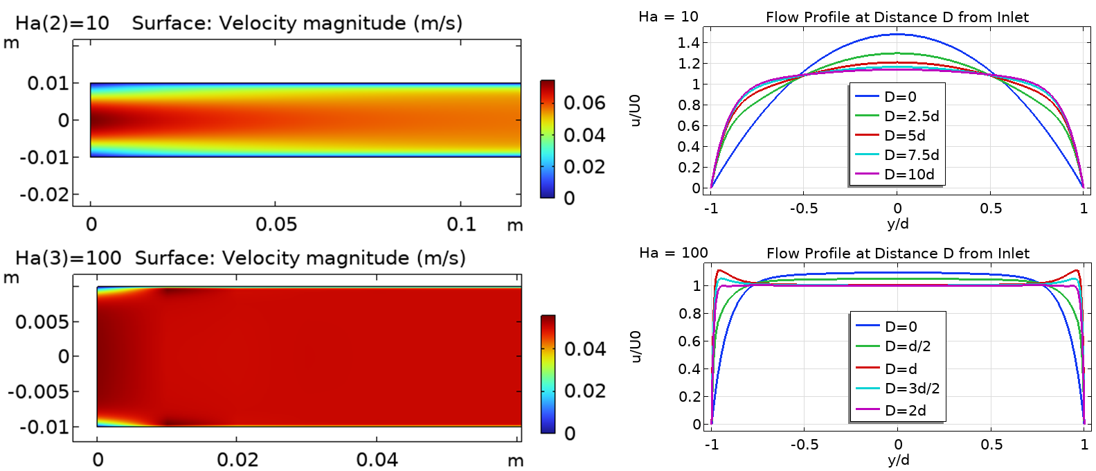
The fluid velocity near the inlet using the Fully developed flow option for Hartmann flow between infinite plates at a Hartmann number of 10 (upper row) and a Hartmann number of 100 (lower row). The left column shows a plot of the magnitude of across the geometry, while the right column plots the normalized velocity on a series of slices across the cross section.

Increasing the distance from the inlet to the area of interest requires the size of the geometry to be increased and enough mesh elements to be generated along the length of the inlet section to resolve the developing flow profile. The number of mesh elements added in this process can be significant due to the small mesh elements needed to resolve the Hartmann layers in the flow. There is then a trade-off between using the Pressure or Mass flow options, which insert the correct flow profile on the inlet but take longer to compute, or using the Fully developed flow option, which is very quick in identifying a flow profile on the inlet but requires additional geometry and degrees of freedom to develop the flow, which slows down the simulation and increases the memory required.

However, as the generated flow profile on the inlet only generates positive fluid velocities, when there is reversed flow in the model, the Fully developed flow profile cannot evolve into the correct magnetohydrodynamic flow profile. In these cases, the Fully developed flow option cannot be used, and the Pressure option must be used instead.

Outlet

The Outlet feature defines a boundary where there is a net flow of fluid out of the model. The standard is to constrain the relative pressure on this boundary to 0, giving the required constraint on for the model to be well defined.

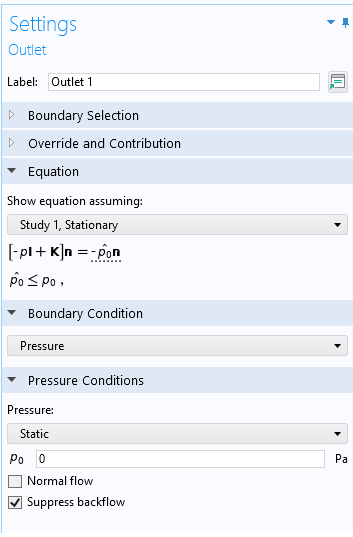
The settings for the Outlet feature, constraining the relative pressure to 0.

As with a pressure type Inlet, if the Suppress backflow option is enabled, instead of treating the pressure as constant on the outlet, it will be allowed to vary across the cross section to prevent backflow. If a constant outlet pressure is required or if the model is expected to exhibit reversed flow, the Suppress backflow option should be disabled.

Azimuthal Flow in 2D Axisymmetric Models

When working in a 2D axisymmetric model, the default settings constrain the flow to be entirely in-plane, removing the azimuthal component of from the equations. This often oversimplifies the system. When it is necessary to include the azimuthal flow in the calculation, the component of the velocity can be returned to the equations by enabling the Swirl flow option in the settings for the Laminar Flow interface.

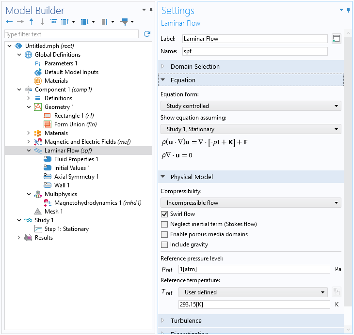
Enabling the Swirl flow option to calculate the azimuthal flow in the system.

With this option enabled, it is possible for motion of the fluid to be driven by a volume force in the fluid, including both the Lorentz force and the drag from the walls of the fluid rotating in the azimuthal direction around the symmetry plane.

In boundary inlets, an azimuthal component can be added to the incident flow, as long as there is also an in-plane flow component. There is no domain inlet option — it is not possible to insert a flow only in the azimuthal direction.

For an introduction to modeling fluid flow using the swirl flow options, see the Swirl Flow Around a Rotating Disk tutorial as well as the downloadable exercise files attached to this article, which focus on building a simple rotational velocity meter using the magnetohydrodynamic effect.