

Eigenfrequency analysis is an integral part of the numerical modeling toolkit. The eigenmodes of a linear system often have distinct qualitative characteristics and evolve differently over a parameter range, such as frequency. We are often asked if there is a way to keep track of and categorize these families of eigenmode solutions over the parameter sweep. In this blog post, we will demonstrate how to do so using the mode overlap integral in the COMSOL Multiphysics® software.
Eigenmodes and the Overlap Integral
Pop quiz: What do designing a fiber optic cable for next-gen communication systems, optimizing the design of a bridge to minimize unwanted mechanical resonance, and perfecting the acoustical layout of your living room all have in common?
In each scenario, we must have a good understanding of the eigenmodes of the system. The eigenmodes, as well as their associated eigenvalues — also called natural frequencies — describe how a linear system would respond to external excitations and thus play a critical role in shaping its design. In certain cases, we want to maximize coupling to one or a few eigenmodes, such as in a cavity filter for radiofrequency communications or in a loudspeaker driver. In other situations, coupling to these resonant modes can lead to catastrophic consequences, like a bridge collapse.
As we tune the parameters of our system, such as operating frequency or geometric dimensions, in a parameter sweep, the eigenmodes and frequencies will naturally change. However, these modes often retain qualitative similarity. As a simple example, let’s take a look at the wave equation on a 2D elliptical membrane — like the vibrating surface of a drumhead or a Chladni plate.
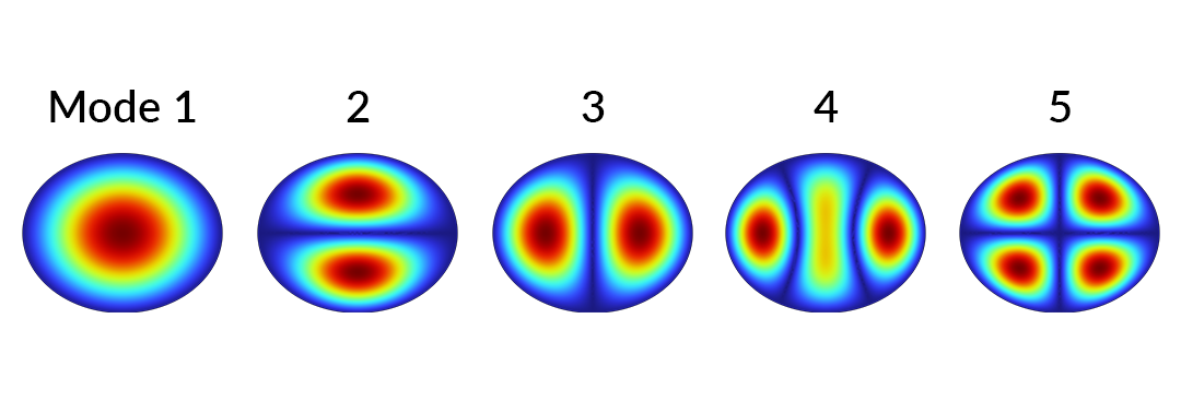
The first five eigenmode solutions of the 2D wave equation on an elliptical membrane with fixed boundaries.
An eigenfrequency study reveals the first five eigenmodes whose displacement magnitudes are shown above. Now, let’s suppose that we want to perform a sweep over the vertical height of the ellipse.
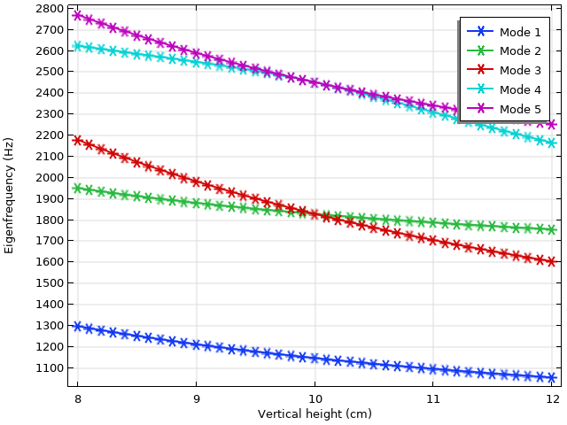
Eigenfrequencies of the first five modes are plotted against the vertical height of the elliptical domain. Note the degeneracies between modes 2 and 3, as well as between modes 4 and 5, at height = 10 cm when the domain is perfectly circular.
The eigenfrequencies of the first five modes are plotted above. Note that when the vertical height is at 10 cm, the model domain is perfectly circular. This results in degeneracies between modes 2 and 3, as well as modes 4 and 5. In fact, past the degenerate point, modes 2 and 3 switch order in the eigenvalue plot. This type of mode-crossing behavior is common in many eigenfrequency studies. How do we keep track of these modes in the eigenvalue plot when their order has shuffled around? To answer this question, let’s take a closer look at one of the modes.
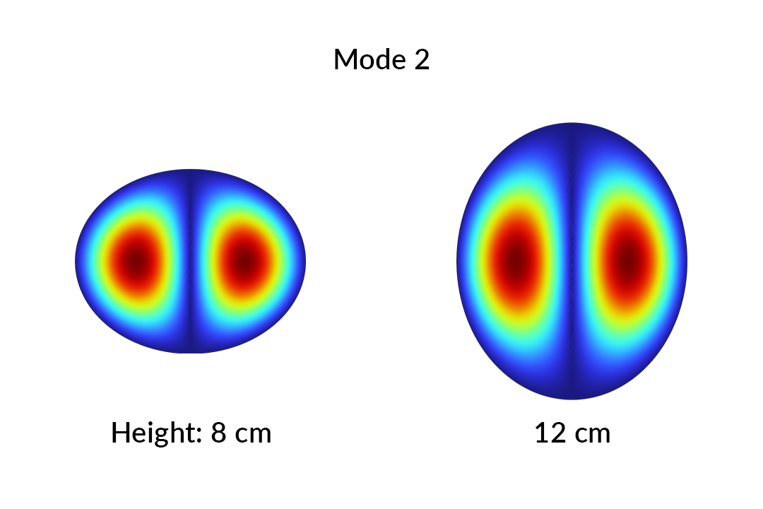
Mode 2 is shown at the two extremes of the parameter range.
Mode 2 is shown above when height = 8 cm and when height = 12 cm. To the human eye, the similarity between the modes are obvious. We can quantify this similarity with the mode overlap integral:
The variables u_i and u_j represent two arbitrary eigenmode solutions. The key part of this equation is in the numerator: we are performing an inner product between the two modes. The denominator normalizes the value of the overlap M to lie between 0 and 1.
The overlap of a mode with itself is 1. The overlap between distinct eigenmodes at the same parameter value is 0, since they are mutually orthogonal. For modes with different parameter values, M will be close to 1 provided the modes are qualitatively similar. For instance, the two modes above have an overlap value of M = 0.95, confirming our visual identification. Two dissimilar modes will have an overlap value close to 0.
With this metric, we can set up a mode matching scheme by imposing a certain threshold on the overlap value. This can be used to filter out or group modes in dispersion plots and even automatically generate mode profile animations with the help of a model method. In the following sections, let’s take a look at applying this strategy to applications in several different physics disciplines.
Example 1: Optically Anisotropic Waveguide
In a previous blog post on how to model optical anisotropic media, we looked at the transverse modes of an optically anisotropic waveguide. These modes can be grouped by the predominant direction of the electric field, as well as the number of amplitude maxima in the transverse plane. A sampling of the E^x_{ij} modes are shown below.
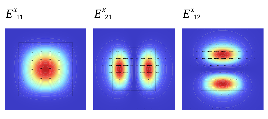
The first three E^x_{ij} eigenmodes in an optically anisotropic waveguide.
Since the primary purpose of the waveguide is to control the flow of light, understanding the behavior of these traveling modes is critical. At each frequency, each mode has an associated effective refractive index that determines how quickly they propagate, their effective wavelength, and how strongly they attenuate (if losses are present in the model). We use the dispersion plot to map out how the effective refractive index changes as a function of frequency.
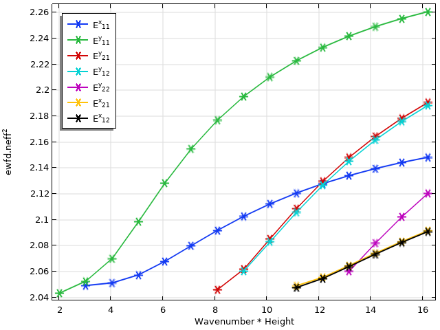
The dispersion plot for the waveguide is shown above. The numerous mode crossings make it necessary to categorize eigenmodes in order to label them correctly.
In the raw output of the mode analysis study, the effective refractive indices are not grouped or ordered in any meaningful way since the solver does not have a priori knowledge of these modes. We apply the overlap integral calculation in order to categorize these eigenvalues by mode profile. Since each effective index value is now associated with a particular E^x_{ij} or E^y_{ij} mode, we can easily make use of filters and plot options to color and annotate each mode in the plot legends. Notice that this method is able to correctly resolve the multiple mode crossings, as well as modes with very close eigenvalues, such as between the E^{x,y}_{12} and E^{x,y}_{21} modes.
Example 2: Eigenfrequencies of a Rotating Blade
Understanding the resonant modes of a rotating component, such as a wind turbine blade or an electric car motor, is critical in applications such as stability analysis or minimizing noise and vibration. As a basic example, let’s take a look at the Fundamental Eigenfrequency of a Rotating Blade model in the Application Library.
As the rectangular blade is rotated at increasing angular velocities, we expect two main competitive phenomena to dominate: stress stiffening and spin softening. The former stiffens the blade due to the stationary stress field from the centrifugal effect and results in an upward influence on the natural frequency. The latter softens the blade due to the radial amplification of motion, thus leading to a downward influence on the natural frequency. The balance of these effects is best portrayed in a Campbell diagram, which is the plot of natural frequencies versus rotational angular velocity.
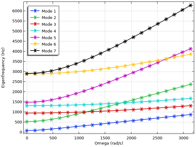
Campbell plot of a rotating blade. Note the significant increase in the eigenfrequencies of modes 2 and 5.
The Campbell plot for the first seven eigenmodes is plotted above. In general, we observe an upward trend in natural frequencies, indicating that stress stiffening plays an outsized role. This is even more pronounced in modes 2 and 5, whose eigenvalues rise dramatically and cross that of other modes over the studied parameter range. The displacement and stresses of the first six modes are shown below.
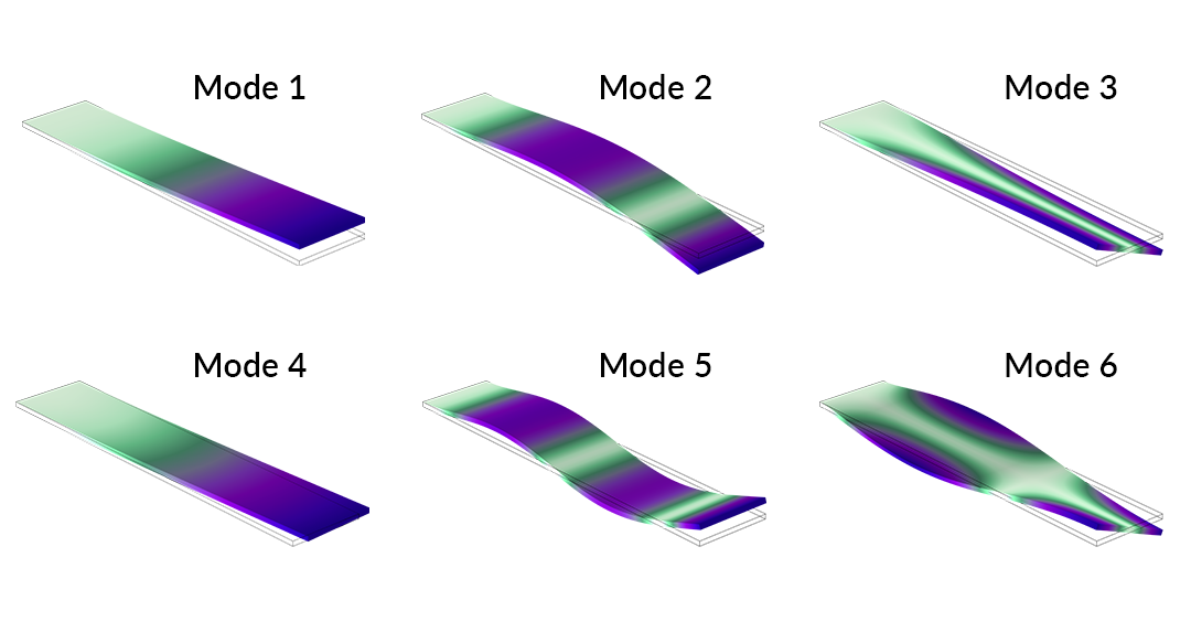
The first six eigenmodes of a rotating blade.
In a more complicated system, the Campbell diagram can be more thickly populated with natural frequencies that exhibit both increasing and decreasing trends. Understanding and visualizing these trends is important, for instance, in determining critical speeds. The mode overlap integral makes it easy to categorize and track the behavior of these mode families.
Example 3: Eigenmodes in a Muffler with Elastic Walls
Multiphysics simulation plays a key role in the design of mufflers for internal combustion engines. On top of modeling pressure waves in the air mass, we also have to take into account the interaction of the air mass with the muffler enclosure. This results in a more accurate transmission profile across the frequency range.
One effect of the acoustic-structure interaction is the introduction of many more resonant modes, as illustrated in these closely related examples: Eigenmodes in a Muffler and Eigenmodes in a Muffler with Elastic Walls. Let’s take a closer look at the latter model. We perform a mode analysis of the muffler cross section over a range of frequencies in order to determine the mode profiles and their corresponding cutoff frequencies.
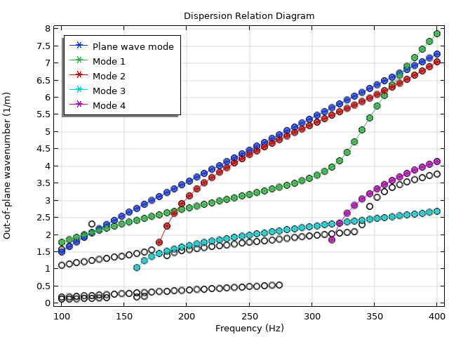
Dispersion plot of the muffler with elastic walls. In addition to the plane wave mode (blue), note the presence of many other mode families due to the acoustic-structure interaction between the air mass and the muffler walls. A subset of them are tracked using the mode overlap method.
A selection of modes and their propagation constants are plotted against frequency in the dispersion diagram above. Clearly, there are trends in the dataset that likely correspond to distinct mode families. For example, the plane wave mode forms a straight diagonal line that cuts across the entire range. By applying the overlap integral, we can confirm the expected behavior of the plane wave mode, as well as track several other modes across the frequency range. These mode profiles are shown below.
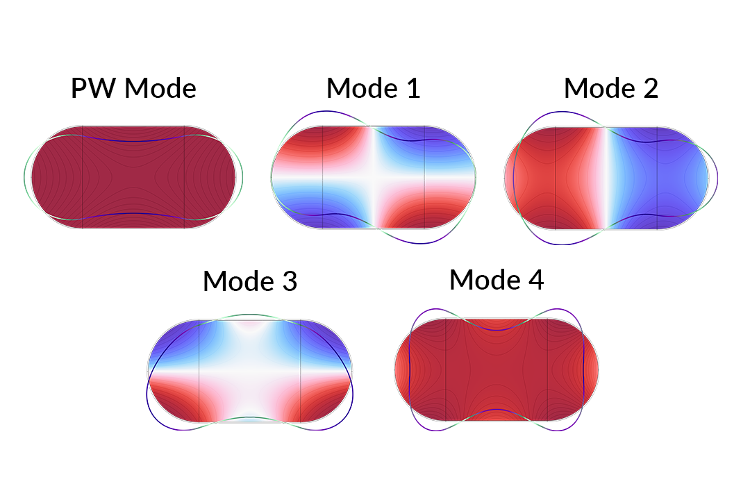
A selection of mode profiles in the muffler with elastic walls are depicted above.
With the help of a model method, we can even automatically generate an animation of the mode evolution across the frequency range.
The evolution of mode 3 is tracked and animated across the parameter range with the help of a model method.
The animation above shows how mode 3 changes dramatically from near its cutoff at 160 Hz to the upper limit of the study at 400 Hz, crossing several other eigenmodes along the way. Tracking the evolution of individual mode families becomes much easier with the help of the mode overlap integral.
Next Steps
In this blog post, we demonstrated the use of the mode overlap integral to help us keep track of and categorize modes in eigenfrequency studies. To get started yourself, click the button below, which will take you to the Learning Center article:
In addition, the models discussed throughout this blog post, can be downloaded in the Application Gallery:
- Optically Anisotropic Waveguide
- Fundamental Frequency of a Rotating Blade
- Eigenmodes in a Muffler with Elastic Walls

Comments (0)